
'%3e%3cpath%20d='M8%200C12.4183%200%2016%203.58172%2016%208C16%2012.4183%2012.4183%2016%208%2016C3.58172%2016%200%2012.4183%200%208C0%203.58172%203.58172%200%208%200ZM11.6162%204.38379C11.2257%203.99337%2010.5927%203.99338%2010.2021%204.38379L8%206.58594L5.79785%204.38379C5.40732%203.99334%204.77429%203.99329%204.38379%204.38379C3.99331%204.77429%203.99335%205.40733%204.38379%205.79785L6.58594%208L4.38379%2010.2021C3.99348%2010.5927%203.99341%2011.2257%204.38379%2011.6162C4.77426%2012.0066%205.40734%2012.0065%205.79785%2011.6162L8%209.41406L10.2021%2011.6162C10.5927%2012.0066%2011.2257%2012.0067%2011.6162%2011.6162C12.0067%2011.2257%2012.0066%2010.5927%2011.6162%2010.2021L9.41406%208L11.6162%205.79785C12.0066%205.40735%2012.0066%204.77429%2011.6162%204.38379Z'%20fill='%23080E17'%20fill-opacity='0.46'/%3e%3c/g%3e%3cdefs%3e%3cclipPath%20id='clip0_3761_713'%3e%3crect%20width='16'%20height='16'%20fill='white'/%3e%3c/clipPath%3e%3c/defs%3e%3c/svg%3e)


'%3e%3cpath%20fill-rule='evenodd'%20clip-rule='evenodd'%20d='M21.4999%2010.9993C21.4999%205.20009%2016.7986%200.498901%2010.9993%200.498901C5.19994%200.498901%200.498657%205.20009%200.498657%2010.9993C0.498657%2016.2404%204.33858%2020.5844%209.35855%2021.3722V14.0346H6.69238V10.9993H9.35855V8.68594C9.35855%206.05427%2010.9262%204.60062%2013.3248%204.60062C14.4736%204.60062%2015.6753%204.80571%2015.6753%204.80571V7.38979H14.3512C13.0468%207.38979%2012.64%208.19921%2012.64%209.0296V10.9993H15.5523L15.0867%2014.0346H12.64V21.3722C17.66%2020.5844%2021.4999%2016.2404%2021.4999%2010.9993Z'%20fill='%231568EA'/%3e%3c/g%3e%3c/svg%3e)


Working with substantial data sets often requires creating links between various sheets, which can be a complex task. VLOOKUP simplifies this process by enabling you to search for a specific value in one sheet and return corresponding data from another. This function is invaluable when you need to consolidate information from different sources, making it easier to analyze and draw insights from your data.
In this article, we will cover various aspects of VLOOKUP, including how to do VLOOKUP in Excel with two spreadsheets, its syntax, and practical examples to illustrate its utility in real-world scenarios. Whether you're working on financial reports, data analysis, or any task involving extensive data sets, mastering VLOOKUP will save you time, improve data accuracy, and enhance your overall efficiency in Excel.

What is the VLOOKUP function?
The VLOOKUP function is a powerful tool in spreadsheet software, like Microsoft Excel or Google Sheets. It stands for "Vertical Lookup" and is used to search for a specific value in a vertical column and retrieve related information from the same row. This excel function is commonly employed for tasks such as data analysis, creating reports, and managing large sets of information. VLOOKUP relies on a key value to locate and return associated data, making it a valuable resource for organizing and processing data efficiently.
Imagine you work in a sales department, and you have a large spreadsheet containing customer data. You want to find detailed information about a particular customer quickly. Instead of manually scrolling through the entire spreadsheet, you can use the VLOOKUP function. For instance, you can search for a customer's name (the key value) and have VLOOKUP retrieve their contact details, order history, and any other relevant information from the same row. This saves you time and ensures accurate data retrieval.
Syntax:
The VLOOKUP function has the following syntax:
VLOOKUP(lookup_value, table_array, col_index_num, [range_lookup])
lookup_value: This is the value you want to search for, such as the customer's name in our example.
table_array: It includes both the table array and the sheet where you want to gather the information. For example, it might appear as "Sheet2!A2:D23", specifying the sheet and the range of data.
col_index_num: This is the column number from which you hope to collect data. It corresponds to the column's position in the table array selected. For instance, if customer contact details are in the second column, you'd use "2" as the col_index_num.
[range_lookup]: This entry is optional, but you can include "TRUE" for approximate matches or "FALSE" for generating an exact match. In our case, if you want an exact customer name match, you'd use "FALSE".
Examples of Using VLOOKUP Function between Two Sheets in Excel
Example 1: Utilizing VLOOKUP Across Two Sheets within a Single Excel Workbook
Let's consider a practical scenario in Excel. We have two sheets in our workbook. The first sheet contains comprehensive employee information, including names, locations, departments, and salaries.

Now, we aim to create a second sheet that displays only salary information. This way, we can share specific salary details with our finance team, such as employee names, unique IDs, and their respective salaries, without revealing all the information.
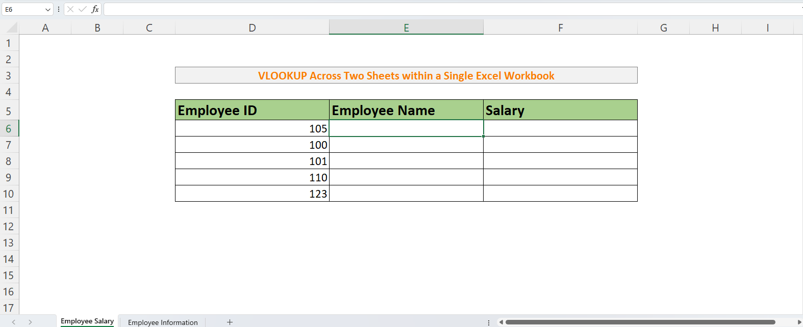
To achieve this, we will leverage the VLOOKUP function. To use the VLOOKUP function effectively, we require a unique identifier, such as an employee's unique ID. With this unique ID, we can employ the VLOOKUP function to search for the corresponding information in the employee information sheet and retrieve the matching data into our new employee salary sheet. Now, let's delve into the process of how do we VLOOKUP between two sheets, here's a comprehensive step-by-step guide:
Let's head over to the "Employee Salary" sheet, where we will deploy the VLOOKUP Function. In cell E6, we will try to fetch the name which corresponds to Employee ID "105" from cell D6.
Step 1: Start by entering "=VLOOKUP(" in cell E6. Always begin with an equal sign to let Excel know that a function is being used.
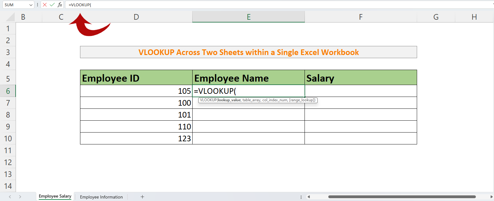
Step 2: For our first argument, which is the "lookup_value", simply select cell D6 because it contains the unique identifier, which is Employee ID.

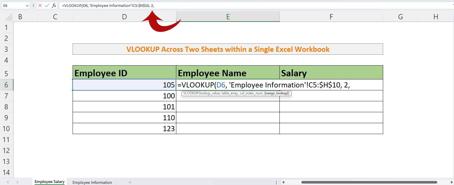
Step 3: Next, we need to define the "table_array". Go to the "Employee Information" sheet and select the entire range, 'Employee Information'!C5:H10. Press F4 to make this an absolute reference so that Excel doesn't change the reference.

Step 4: Now, we need to specify to Excel which column to perform the VLOOKUP on, i.e., the order in the table. Since we want to fetch the employee name, and it's in the 2nd column in the "Employee Information" sheet, we'll enter "2" in the "col_index_num" argument.
Step 5: The last argument is the [range_lookup]. Here, we will select "FALSE" because we want an exact match. If this is not clear, refer back to the information provided in the article regarding each argument.
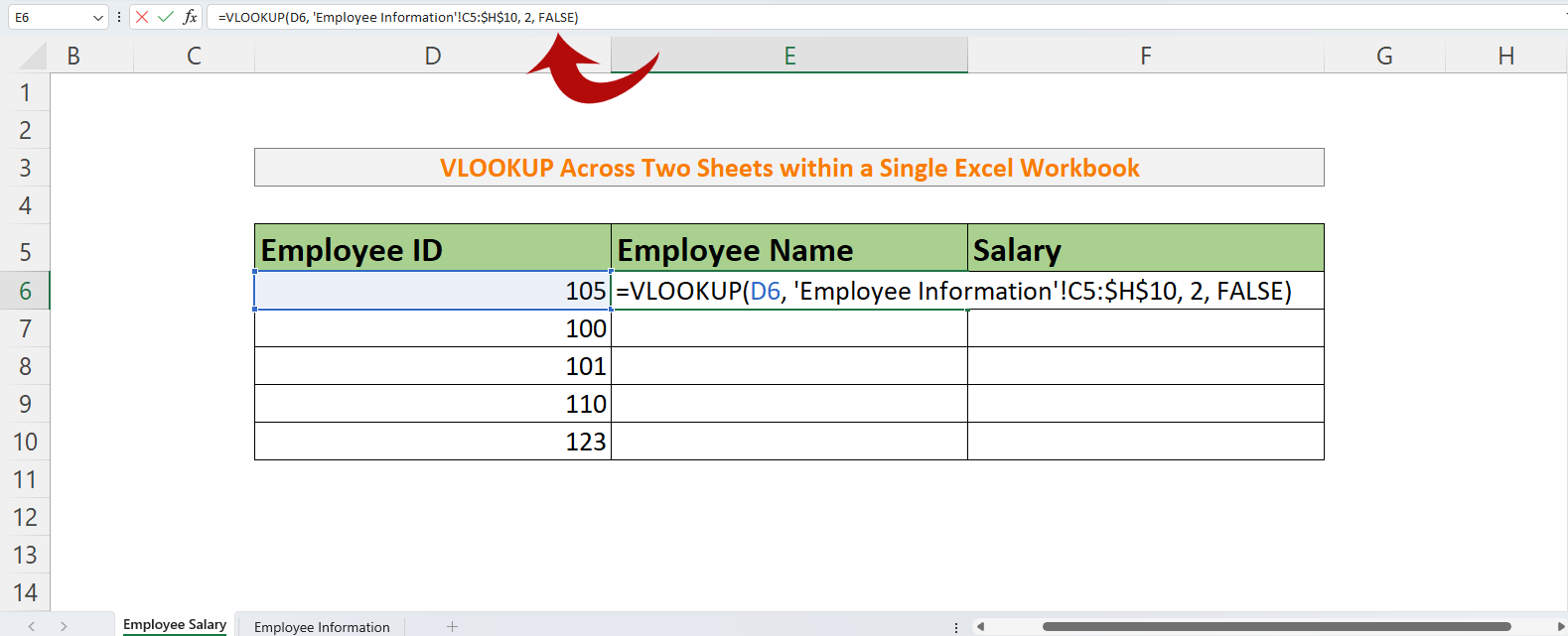
Step 6: Now that our VLOOKUP function is complete, simply press "ENTER". Excel will perform the VLOOKUP function across two sheets in the same workbook, and we will get our result. We can then copy the formula for other cells using the "Fill Handle" to obtain the results.
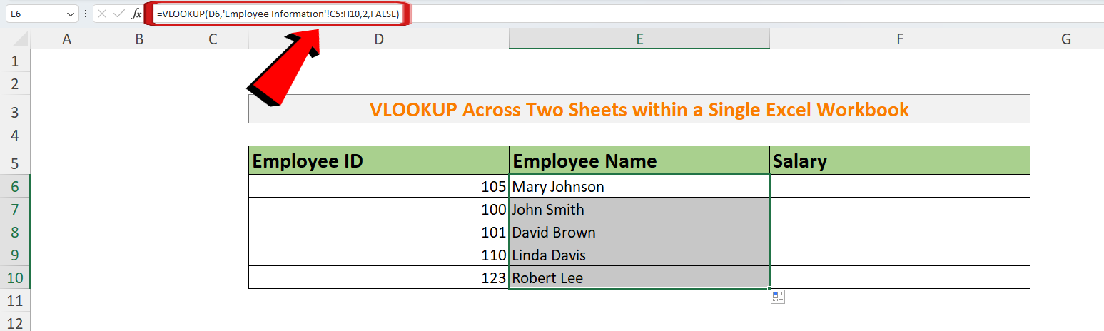
We will be using the same VLOOKUP function for our Salary column with only one minor change, which is our 3rd argument: "col_index_num," which will now be "4".

Example 2: Using VLOOKUP Across Two Sheets in Different Workbooks
Imagine you have data in two different workbooks, and you need to extract information from one workbook into another. You can effortlessly achieve this using the VLOOKUP function. Let's dive into a practical example:
Workbook 1 contains detailed product information, including product names, categories, prices, and quantities in stock.

Workbook 2 aims to create a summary of products and their prices for reporting purposes.

Open Workbook 2 and navigate to the sheet where you want to display the product prices. In cell F7, we will use VLOOKUP to fetch the price of a specific product.
Step 1: Start by entering "=VLOOKUP(" in cell F7. Begin with an equal sign to indicate you are using a function.

Step 2: For the "lookup_value" (first argument), select the cell that contains the product name you want to search. In this case, it's cell E7, where we want to find the price for the product named "Widget A".

Step 3: The "table_array" (second argument) is where we specify where to search for the product price. Navigate to Workbook 1 and the corresponding sheet that holds the product information. Select the entire range, e.g., 'Products'!D5:G15, and press F4 to make it an absolute reference.
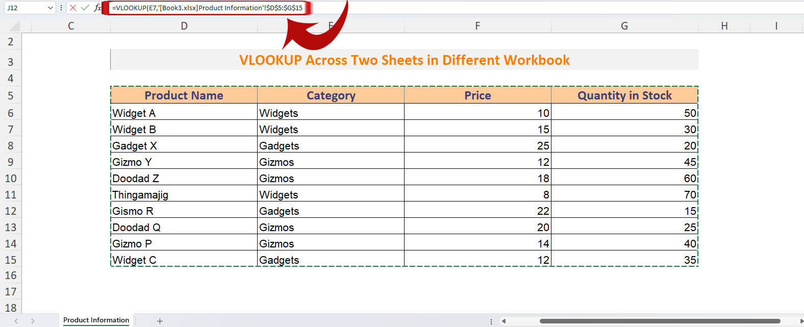
Step 4: For the "col_index_num" (third argument), specify which column contains the data you want to retrieve. In this scenario, prices are in the second column of the “Products” sheet, so enter "2".

Step 5: The [range_lookup] (fourth argument) is set to "FALSE" to ensure an exact match.
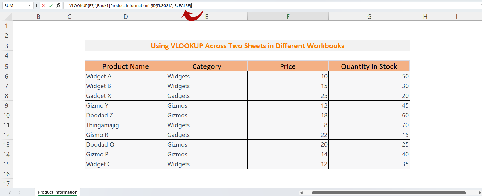
Step 6: Your VLOOKUP function is now complete. Press "ENTER", and Excel will perform the VLOOKUP function between the two workbooks, extracting the price of "Widget A" into cell B2.
Step 7: To apply this function to other products, simply drag the fill handle (the small square at the bottom-right of the cell) down the column to copy the formula for other products. Excel will automatically adjust the references.
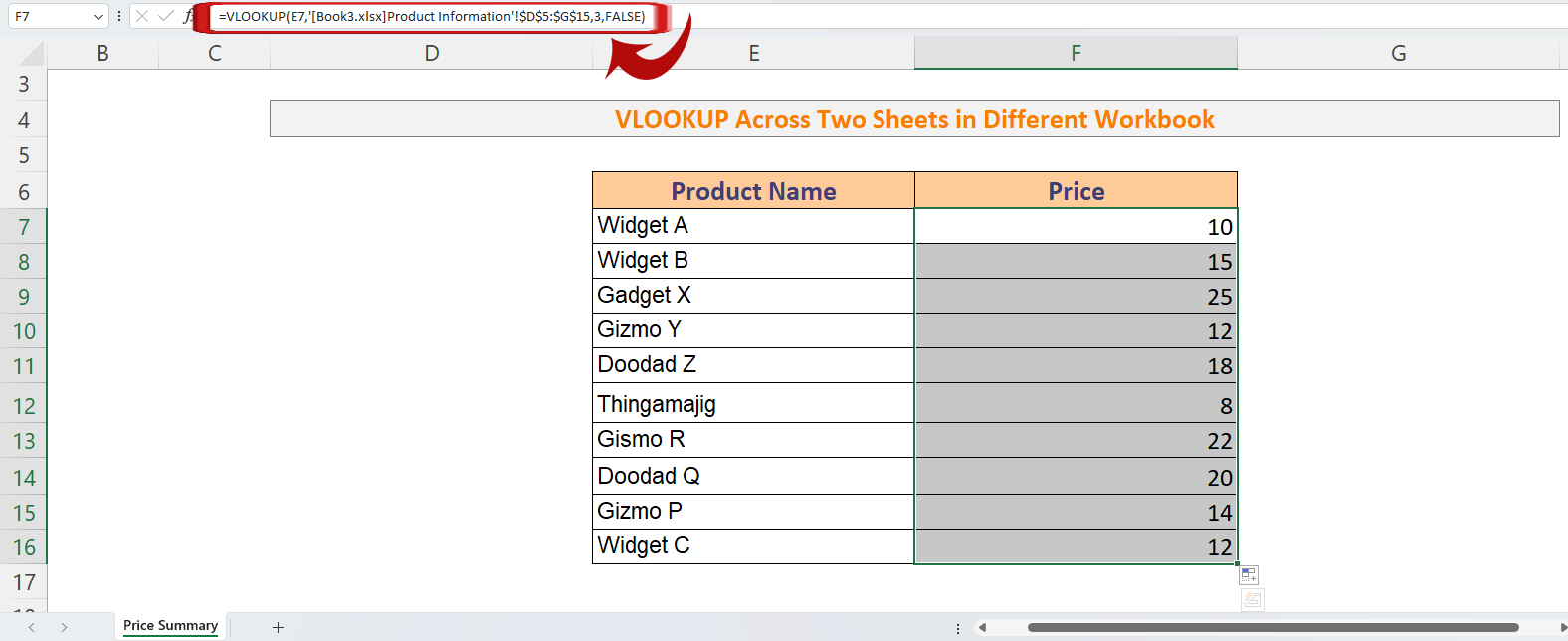
Step 8: You can now see the product prices populated in Workbook 2, retrieved from Workbook 1, making it easier to generate your reports.
That's it! You've successfully learned how to use VLOOKUP across two sheets in different workbooks to streamline your data management tasks..
Best Alternative to Excel—WPS Office
Why Choose WPS Office
WPS Office is not just the cost-effective, user-friendly sibling of Microsoft Office, but it also stands as the most compelling alternative to Excel, a heavyweight in the spreadsheet software arena. With its comprehensive features and compatibility, WPS Office emerges as a formidable contender for users seeking a reliable, accessible, and powerful spreadsheet tool. Its ability to seamlessly handle data manipulation, analysis, and presentation positions it as the best alternative to Excel for a wide range of users. Whether you're a business professional, student, or anyone in need of spreadsheet capabilities, WPS Office offers a compelling solution.

The software's ability to seamlessly handle various spreadsheet tasks, from data entry to complex analysis, contributes to its popularity among professionals and casual users alike. WPS Office stands out not only as a competent alternative to Excel but also as a practical and reliable tool for all your data management, editing, and analytical needs.
How to Use Vlookup between Two Sheets in WPS Office
Let's explore a unique example of how to use the VLOOKUP function in WPS Office, combined with the AVERAGE function. We'll be creating a spreadsheet to calculate the final grade for students, which we'll call the "Final Grade".
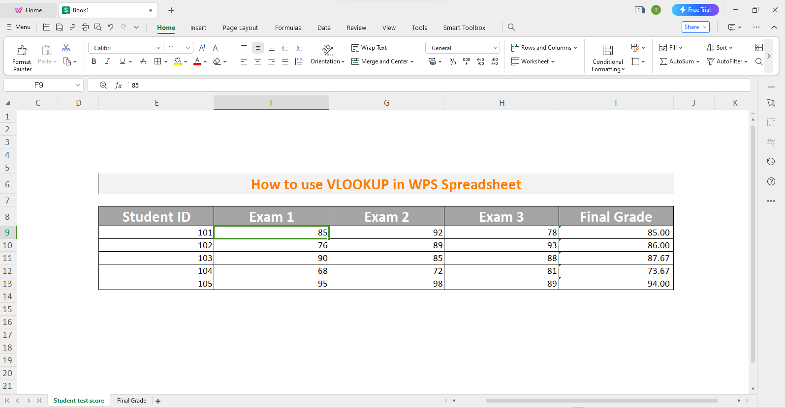
We have a "Student Test Score" sheet that contains students' exam scores and their final grades.
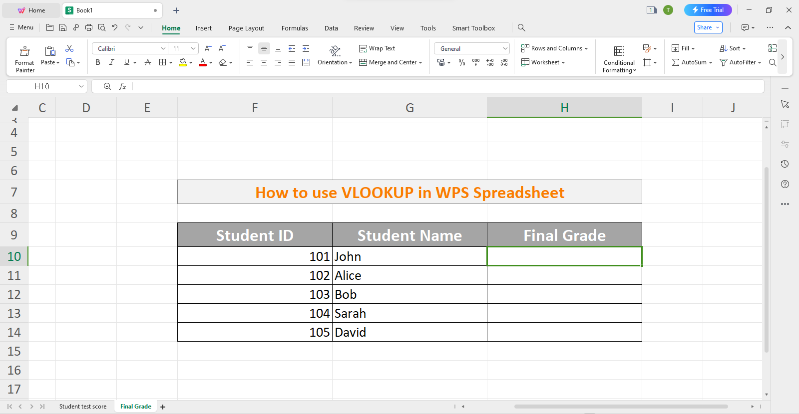
To begin, open the "Final Grade" sheet, we will be using the VLOOKUP function to fetch the final grade from the "Student Test Score" sheet.
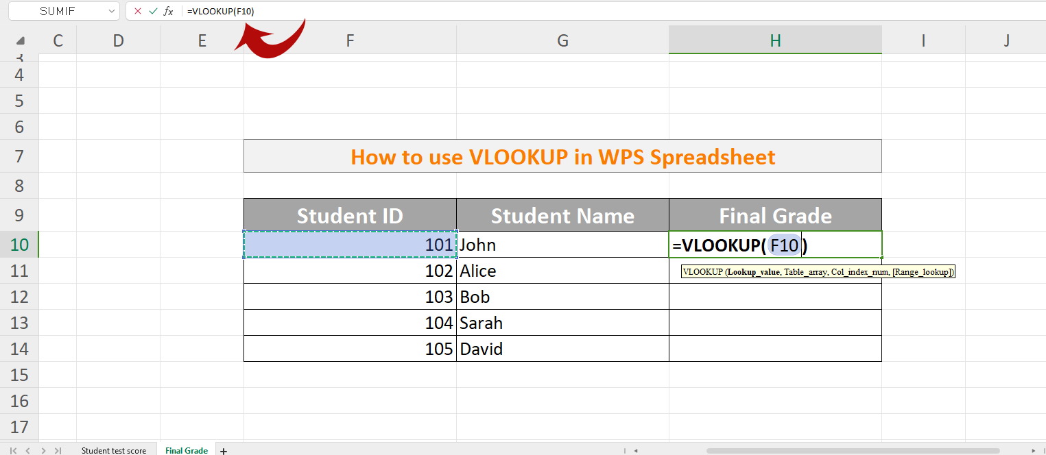
Step 1: Initiate the VLOOKUP function by typing "=VLOOKUP()" in cell H10. Notice how the parentheses are automatically added to prevent errors.

Step 2: For the lookup_value argument, use the unique Student ID from cell F10.
Step 3: Now, we need to specify the table_array. To do this, navigate to the "Student Test Score" sheet and select the entire table, pressing F4 to make it an absolute reference.

Step 4: Next, choose the col_index_num. Instead of switching back to the "Student Test Score" sheet, WPS Office displays the columns under the formula to make it convenient. Select the "Final Grade", which is the 5th column.

Step 5: For the last argument, which is range_lookup, select "FALSE" to ensure an exact match.

Step 6: Since the closing parenthesis is already there by default, press "Enter" to get the results. Then, use the "Auto Fill" handle to copy the formula to other cells.

This process is simple and user-friendly, with WPS Spreadsheet enhancing the user experience by adding parentheses and showing columns for easy selection.
Example- VLOOKUP in combination with AVERAGE Function
Now, let's make things more interesting. Suppose the "Student Test Score" sheet doesn't have the final grade, and we need to calculate it using VLOOKUP in combination with the AVERAGE function.

A quick overview of the AVERAGE function: It calculates the average of a range of cells.
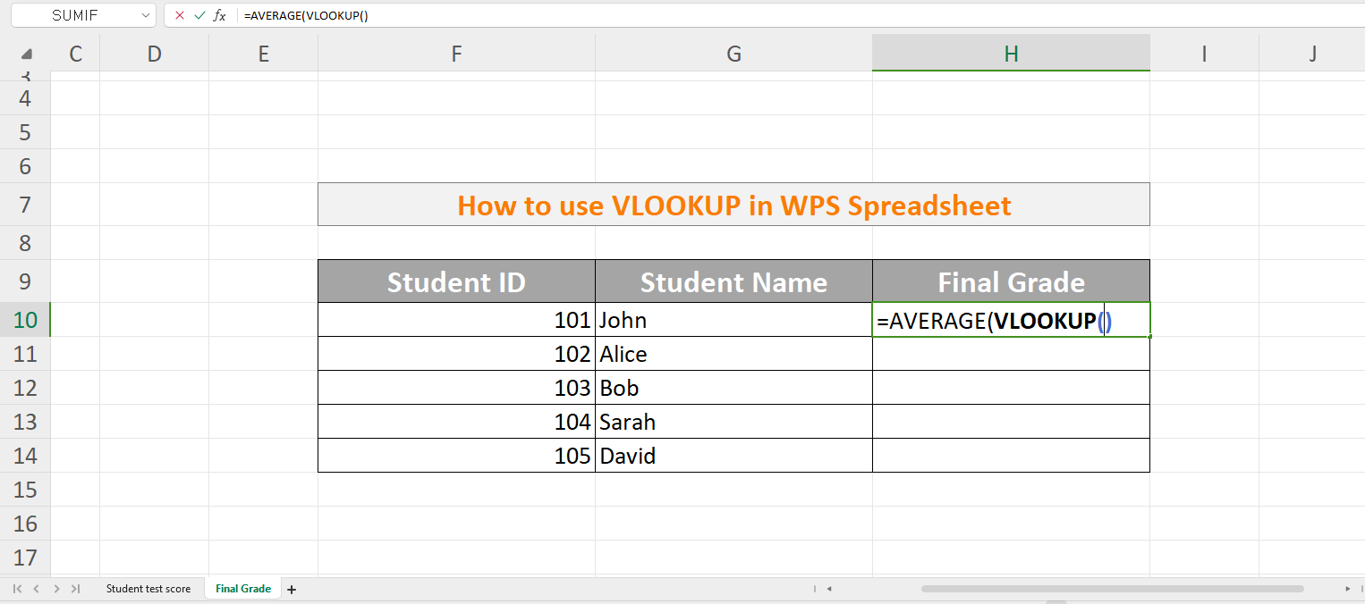
Step 1: Return to the "Final Grade" sheet and enter the AVERAGE function in cell H10: "=AVERAGE()".

Step 2: Now, nest the VLOOKUP function inside the AVERAGE function. Since we have three exam scores, we'll use VLOOKUP three times.
Step 3: Similar to our VLOOKUP earlier, the student ID will be the lookup_value. Select cell F10.
Step 4: For the table_array, choose the table from the "Student Test Score" sheet and press F4 to make it an absolute reference.

Step 5: Here's where it differs. For the first VLOOKUP, we're fetching the Exam 1 score, so select column 2 and choose "FALSE" for the last argument to complete the first VLOOKUP.

Step 6: To begin the next VLOOKUP, add a comma as a separator and then enter "VLOOKUP" again.
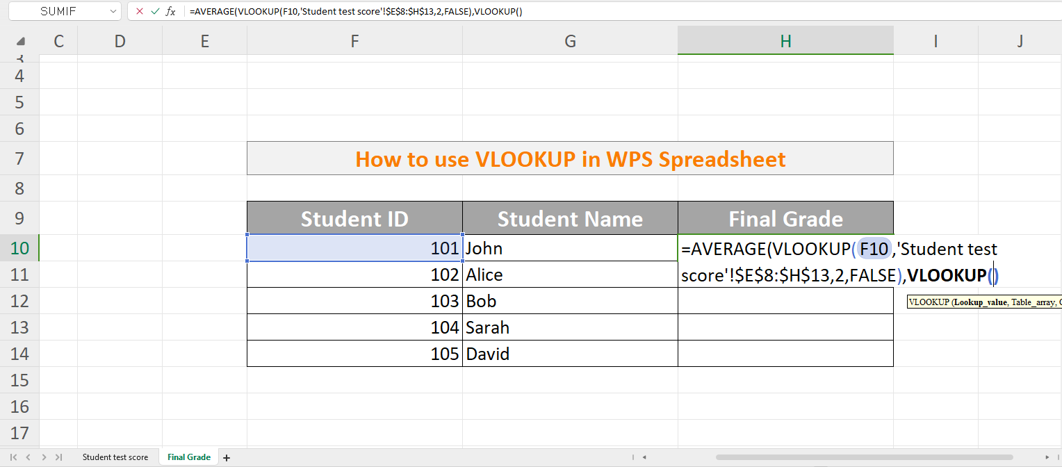
Step 7: For the next two VLOOKUPs, follow the same steps. The only change is the "col_index_num" for Exam 2 and Exam 3 scores.

Step 8: Add a parenthesis to complete the AVERAGE function and press "Enter" for the results. To copy the function to other cells, use the Autofill handle.
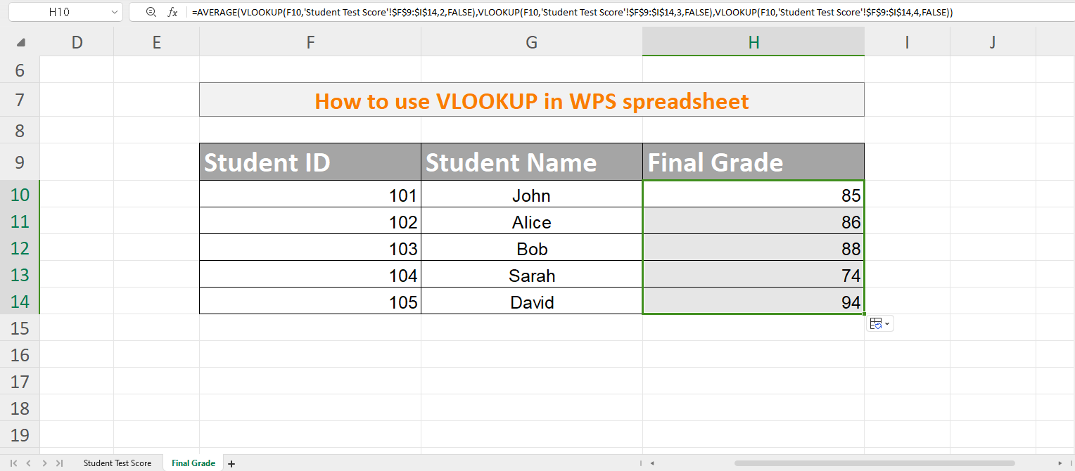
And there you have it, the final grade calculated using the VLOOKUP function nested within the AVERAGE function. What's noteworthy is how WPS Spreadsheet simplifies a potentially lengthy and complex process with these additional features. Try WPS Spreadsheet for yourself; this tool can be a valuable asset for your spreadsheet tasks.


FAQs
Q1. Can I use VLOOKUP to compare two columns?
VLOOKUP is a powerful Excel function that allows you to quickly and easily compare data across two columns, making it useful for data reconciliation, error detection, and learning from related data points. Its versatility allows for comprehensive data analysis and informed conclusions.
Q2. How do I pull data from another sheet in Excel?
To pull data from another sheet in Excel, follow these straightforward steps:
Step 1: Launch Excel and access the sheet where you want the data.
Step 2: Choose the exact cell in which you want the information to appear.
Step 3: In that cell, type an equal sign "=".
Step 4: Now, right away, insert the name of the source sheet, accompanied by an exclamation mark, and then the name of the cell containing the data you want to pull. For example, it would look like this: "=SourceSheetName!A2".
Step 5: Press Enter. The data from the cell in the source sheet will appear in your chosen cell.
Start Your VLOOKUP Journey Today
By mastering VLOOKUP, you can streamline your data-related tasks, minimize errors, and improve your efficiency. The ability to establish dynamic connections between sheets and extract data seamlessly is an invaluable skill for data analysts, financial professionals, and Excel enthusiasts. If you're ready to explore how to do VLOOKUP in Excel with two spreadsheets, we recommend considering WPS Office. as a valuable companion in your data-related tasks.
WPS Office offers a user-friendly and cost-effective alternative to Microsoft Office, including a robust spreadsheet tool that can simplify your data management and analysis. With WPS Office, you can efficiently handle large data sets, collaborate on complex projects, and make the most of functions like VLOOKUP. Download WPS Office now and experience its numerous benefits in streamlining your data work.

'%3e%3cpath%20d='M19.9911%204.11386V6.471H18.5894C18.0775%206.471%2017.7322%206.57814%2017.5536%206.79243C17.3751%207.00671%2017.2858%207.32814%2017.2858%207.75671V9.44421H19.9019L19.5536%2012.0871H17.2858V18.8639H14.5536V12.0871H12.2769V9.44421H14.5536V7.49779C14.5536%206.39064%2014.8632%205.53201%2015.4822%204.92189C16.1013%204.31177%2016.9257%204.00671%2017.9554%204.00671C18.8304%204.00671%2019.509%204.04243%2019.9911%204.11386Z'%20fill='%23333333'/%3e%3c/g%3e%3cdefs%3e%3cclipPath%20id='clip0_2938_8199'%3e%3crect%20width='16'%20height='16'%20fill='white'%20transform='translate(8%204.00671)'/%3e%3c/clipPath%3e%3c/defs%3e%3c/svg%3e)
'%3e%3cpath%20d='M17.5237%2010.7813L23.4811%204H22.0699L16.8949%209.88693L12.7648%204H8L14.2469%2012.9029L8%2020.0133H9.4112L14.8725%2013.7952L19.2352%2020.0133H24M9.92053%205.04213H12.0885L22.0688%2019.0224H19.9003'%20fill='%23333333'/%3e%3c/g%3e%3cdefs%3e%3cclipPath%20id='clip0_2938_8200'%3e%3crect%20width='16'%20height='16.0134'%20fill='white'%20transform='translate(8%204)'/%3e%3c/clipPath%3e%3c/defs%3e%3c/svg%3e)


