
'%3e%3cpath%20d='M8%200C12.4183%200%2016%203.58172%2016%208C16%2012.4183%2012.4183%2016%208%2016C3.58172%2016%200%2012.4183%200%208C0%203.58172%203.58172%200%208%200ZM11.6162%204.38379C11.2257%203.99337%2010.5927%203.99338%2010.2021%204.38379L8%206.58594L5.79785%204.38379C5.40732%203.99334%204.77429%203.99329%204.38379%204.38379C3.99331%204.77429%203.99335%205.40733%204.38379%205.79785L6.58594%208L4.38379%2010.2021C3.99348%2010.5927%203.99341%2011.2257%204.38379%2011.6162C4.77426%2012.0066%205.40734%2012.0065%205.79785%2011.6162L8%209.41406L10.2021%2011.6162C10.5927%2012.0066%2011.2257%2012.0067%2011.6162%2011.6162C12.0067%2011.2257%2012.0066%2010.5927%2011.6162%2010.2021L9.41406%208L11.6162%205.79785C12.0066%205.40735%2012.0066%204.77429%2011.6162%204.38379Z'%20fill='%23080E17'%20fill-opacity='0.46'/%3e%3c/g%3e%3cdefs%3e%3cclipPath%20id='clip0_3761_713'%3e%3crect%20width='16'%20height='16'%20fill='white'/%3e%3c/clipPath%3e%3c/defs%3e%3c/svg%3e)


'%3e%3cpath%20fill-rule='evenodd'%20clip-rule='evenodd'%20d='M21.4999%2010.9993C21.4999%205.20009%2016.7986%200.498901%2010.9993%200.498901C5.19994%200.498901%200.498657%205.20009%200.498657%2010.9993C0.498657%2016.2404%204.33858%2020.5844%209.35855%2021.3722V14.0346H6.69238V10.9993H9.35855V8.68594C9.35855%206.05427%2010.9262%204.60062%2013.3248%204.60062C14.4736%204.60062%2015.6753%204.80571%2015.6753%204.80571V7.38979H14.3512C13.0468%207.38979%2012.64%208.19921%2012.64%209.0296V10.9993H15.5523L15.0867%2014.0346H12.64V21.3722C17.66%2020.5844%2021.4999%2016.2404%2021.4999%2010.9993Z'%20fill='%231568EA'/%3e%3c/g%3e%3c/svg%3e)


Unlock the full potential of Excel with the power of filtering. In this guide, we address the common challenge of efficiently using filters to extract the data you need. Discover the secrets to effortless filtering and make data manipulation a breeze. Ready to dive in? Let's master the art of Excel filtering together. And for a seamless experience, don't forget to explore WPS Office - your free and convenient ally in data management.
Part 1. 2 Methods to Filter in Excel
#1 Filter Data in Tables in Excel
You'll also come across many excel functions, allowing you to streamline complex data analysis even further. Filtering data is a powerful technique in Excel that allows you to quickly extract specific information from large datasets. In this tutorial, we will explore three different cases of filtering - filtering by value, by color, and by text. Follow the step-by-step instructions and leverage the full potential of Excel's filtering capabilities.
Filter by value
To filter data by value, you need to follow these steps:
Step 1 Select the range of cells that you want to filter.

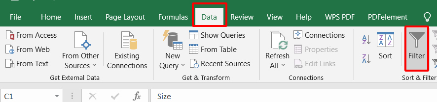
Step 2 Click on the Data tab. In the Sort & Filter group, click on the Filter button.
Step 3 In the Filter by value drop-down list, select the criteria that you want to use to filter the data.

Step 4 The column will be subjected to the filter.
Filter by color
To filter data by color, you need to follow these steps:
Step 1 Select the range of cells that you want to filter.

Step 2 Click on the Data tab. In the Sort & Filter group, click on the Filter button.

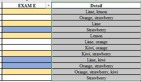
Step 3 In the Filter by color drop-down list, select the color that you want to filter by.

Step 4 The filter will be applied to the column.

Filter by text
To filter data by text, you need to follow these steps:
Step 1 Select the range of cells that you want to filter.
Step 2 Click on the Data tab. In the Sort & Filter group, click on the Filter button.

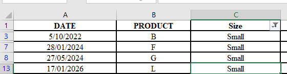
Step 3 In the Filter by text drop-down list, select the criteria that you want to use to filter the data.

Or Enter the text that you want to filter by in the Value box.

Step 4 Click on the OK button.
#2 Use Filter Formula in Excel
You may use the FILTER function to filter a set of data depending on criteria you provide.
Step 1 Select a cell where you want to enter the filter formula.
Step 2 In the following example, we used the formula =FILTER(A5:D20,C5:C20=H2,"") to return all entries for Apple, as specified in cell H2, and an empty string ("") if no apples were found.

Part 2. Best Alternative - WPS Office

What is WPS Office
WPS Office is a sophisticated office suite with several features for efficiency and creativity. It comprises a word processor, spreadsheet software, presentation software, and other tools. WPS Office is Microsoft Office compatible, so you can quickly open and edit files generated in Microsoft Office. It also provides clear instructions to assist you in resolving any issues that may arise.


How to Filter in WPS Office
The filter function in WPS Office allows you to filter data based on a set of criteria. This can be useful for finding specific data, such as rows that contain a particular value or rows that meet certain conditions.
How to Add a Filter in Excel
Step 1 Open WPS Spreadsheet
Step 2 Select the Data Range

Click on any cell within the data range you want to filter.
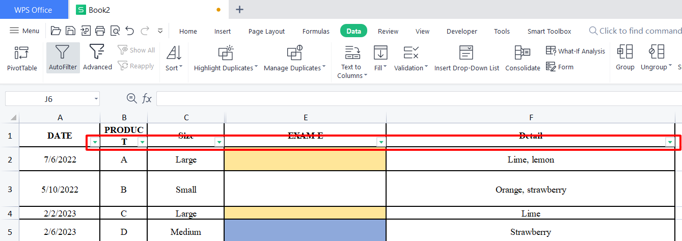
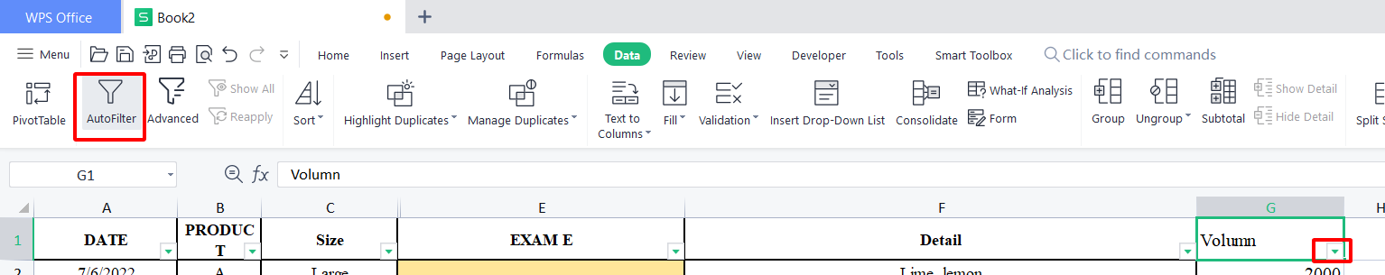
Step 3 Go to the "Data" tab on the Excel ribbon at the top of the window. In the "Sort & Filter" group, you'll find a button labeled "AutoFilter." Click on it to enable the filter for the selected data range.
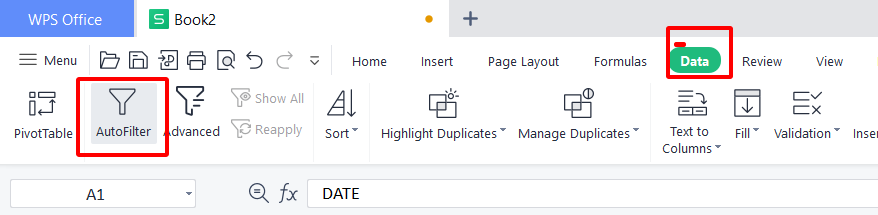
Step 4 Once you enable the filter, you will see small filter arrows appear next to the column headers in the data range. These arrows indicate that the filter is active.
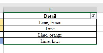
Filter data in a table
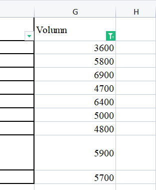
Step 1 Choose the column header arrow for which you wish to filter. Then uncheck (Select All)

Step 2 To proceed, select the checkboxes you wish to see. Press the OK button.

The column header arrow will transform to a filter icon. Before modifying or removing the filter, you must first pick this icon.

You may make your worksheets appear more professional by following these tips. If you wish to see all of the values in a spreadsheet, you may undo the filter.
How to Add a Filter in Excel for a Column
Step 1 Choose the column to filter by clicking on the matching letter at the top.
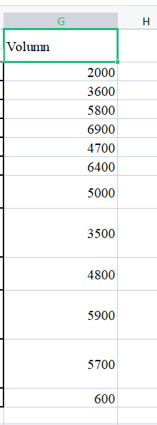
Step 2 Then, in the toolbar at the top, select Data. Then, on the top toolbar, click on Filter. An arrow will appear at the top of the column.
Step 3 You must click the arrow at the top of the column. The Filters pop-up window will appear. Then, click Numeric Filters to see a more thorough pop-up box. Click OK after selecting the filtering option. The sheet will be filtered for data more than 3500 in this case.


FAQs
1. What is the fastest way to filter in Excel?
The easiest ways to filter are to choose values from a list and to search. When you click the arrow in a filterable column, all values in that column display in a list. Clear the (pick All) check box in the list to pick by values.
2. Can you use multiple filters at the same time in Excel?
You can apply multiple filters to as many columns as you wish, not just two. You may go one step further and apply another filter to the "state" column. We have the third filter on the column "state" in the preceding example, where we have filtered all the entries with CA.
3. How Do I See all Filters in an Excel Spreadsheet?
Simply click on the filter drop-down arrow to see which filters have been applied to a column. This will give a list of all the filters applied to the column. A checkmark will appear next to any filters that are presently active.
4. What is the Shortcut for Filtering in Excel?
AutoFilter: Ctrl + Shift + L
Clear Filter: Alt + Down Arrow
Filter by Selection: Ctrl + Shift + L (twice)
Filter by Color: Alt + H + L
Filter by Top/Bottom Values: Alt + A + S
Filter by Date: Ctrl + Shift + #
Filter by Text: Ctrl + Shift + $
Filter by Multiple Criteria: Ctrl + Shift + A
Toggle Filter On/Off: Ctrl + Shift + L
Clear All Filters: Alt + A + C
These shortcuts will help you work efficiently with data filtering in Excel. Use them to quickly apply filters, clear filters, and perform various types of data filtering in your worksheets.
5. How to Remove the Filter in Excel?
To remove all filters from a worksheet, use one of the following methods:
Select Clear the Sort & Filter group from the Data tab.
Select Sort & Filter > Clear from the Home tab > Editing group.
Summary
In this tutorial, we learned how to efficiently use Excel's filter function to extract specific data from large datasets. By filtering data based on value, color, and text, we can quickly find the information we need, streamlining data analysis and enhancing productivity.
If you're looking for a reliable and user-friendly office suite that seamlessly works with Microsoft Office filesI highly recommend giving WPS Office a try. With its seamless compatibility with Microsoft Office files and user-friendly interface, it streamlines data management and boosts productivity.

'%3e%3cpath%20d='M19.9911%204.11386V6.471H18.5894C18.0775%206.471%2017.7322%206.57814%2017.5536%206.79243C17.3751%207.00671%2017.2858%207.32814%2017.2858%207.75671V9.44421H19.9019L19.5536%2012.0871H17.2858V18.8639H14.5536V12.0871H12.2769V9.44421H14.5536V7.49779C14.5536%206.39064%2014.8632%205.53201%2015.4822%204.92189C16.1013%204.31177%2016.9257%204.00671%2017.9554%204.00671C18.8304%204.00671%2019.509%204.04243%2019.9911%204.11386Z'%20fill='%23333333'/%3e%3c/g%3e%3cdefs%3e%3cclipPath%20id='clip0_2938_8199'%3e%3crect%20width='16'%20height='16'%20fill='white'%20transform='translate(8%204.00671)'/%3e%3c/clipPath%3e%3c/defs%3e%3c/svg%3e)
'%3e%3cpath%20d='M17.5237%2010.7813L23.4811%204H22.0699L16.8949%209.88693L12.7648%204H8L14.2469%2012.9029L8%2020.0133H9.4112L14.8725%2013.7952L19.2352%2020.0133H24M9.92053%205.04213H12.0885L22.0688%2019.0224H19.9003'%20fill='%23333333'/%3e%3c/g%3e%3cdefs%3e%3cclipPath%20id='clip0_2938_8200'%3e%3crect%20width='16'%20height='16.0134'%20fill='white'%20transform='translate(8%204)'/%3e%3c/clipPath%3e%3c/defs%3e%3c/svg%3e)


