Free All-in-One Office Suite with PDF Editor
Edit Word, Excel, and PPT for FREE.
Read, edit, and convert PDFs with the powerful PDF toolkit.
Microsoft-like interface, easy to use.
Windows • MacOS • Linux • iOS • Android

Catalog
IRR Function in EXCEL
· Description:
IRR means the Internal Rate of Return that is represented by numbers for a series of cash flows. It requires that the cash flows are at regular intervals.
· Syntax:
(Value, guess)
· Arguments:
Value is an array or a reference to cells that contain numbers for which you want to calculate the internal rate of return.
Guess is a number that you guess is close to the result of IRR; 0.1 (10 percent) of omitted.
· Example:
Suppose we want to calculate the IRR of this investment project with an initial investment of 50,000 and a yearly income of 8000. The initial investment (-50,000) is negative because it is expenditure. The cash flow in the following year (8,000) is a positive value because it is income.
1. Open your table in WPS Spreadsheet
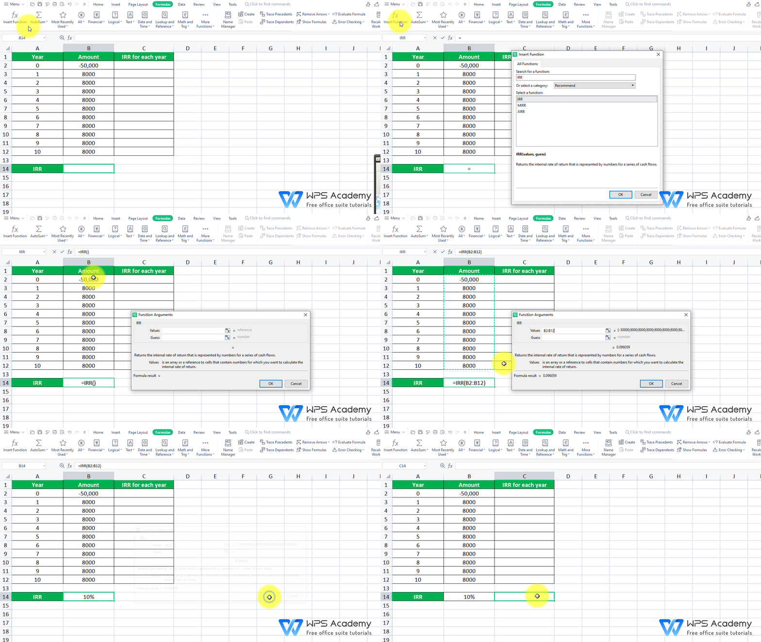
2. Select cell B14 where we want to insert the function. Then head to the Formulas tab > Insert Function > enter IRR in the edit box, or just type“=IRR”in the cell.
3. Here we need to insert the IRR function.
1) Value is an array or a reference to cells that contain numbers for which you want to calculate the internal rate of return. B2:B12 is the area that contains the cash flow amounts.
2) Guess is a number that you guess is close to the result of IRR. The second argument is a guessed number that is close to the expected internal rate of return, which we choose to omit.
So, in the pop-up dialog, enter B2:B12 at Value. Then click OK.
We can get 10% as the result, which is the IRR of this investment project would give after 10 years.

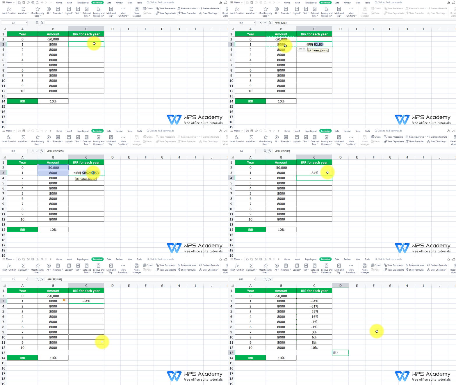
4. We can also calculate the IRR for each year. Click cell C3 where we want to get the IRR for year 1 with the IRR function.
1)Value: B2:B3 is the cash flow amounts of the first year. Also, we need to press F4 to make cell B2 an absolute reference because we don’t want it to change when dragging down cell C3, meanwhile we need to make cell B3 a relative reference because we need it to update.
2) Guess is a number that you guess is close to the result of IRR. The second argument is a guessed number that is close to the expected internal rate of return, which we choose to omit.
So, we enter the function “=IRR($B$2:B3)”.
5. Hove over cell C3, and drag it all the way down. Now we get the IRR for each of the ten years.


