
'%3e%3cpath%20d='M8%200C12.4183%200%2016%203.58172%2016%208C16%2012.4183%2012.4183%2016%208%2016C3.58172%2016%200%2012.4183%200%208C0%203.58172%203.58172%200%208%200ZM11.6162%204.38379C11.2257%203.99337%2010.5927%203.99338%2010.2021%204.38379L8%206.58594L5.79785%204.38379C5.40732%203.99334%204.77429%203.99329%204.38379%204.38379C3.99331%204.77429%203.99335%205.40733%204.38379%205.79785L6.58594%208L4.38379%2010.2021C3.99348%2010.5927%203.99341%2011.2257%204.38379%2011.6162C4.77426%2012.0066%205.40734%2012.0065%205.79785%2011.6162L8%209.41406L10.2021%2011.6162C10.5927%2012.0066%2011.2257%2012.0067%2011.6162%2011.6162C12.0067%2011.2257%2012.0066%2010.5927%2011.6162%2010.2021L9.41406%208L11.6162%205.79785C12.0066%205.40735%2012.0066%204.77429%2011.6162%204.38379Z'%20fill='%23080E17'%20fill-opacity='0.46'/%3e%3c/g%3e%3cdefs%3e%3cclipPath%20id='clip0_3761_713'%3e%3crect%20width='16'%20height='16'%20fill='white'/%3e%3c/clipPath%3e%3c/defs%3e%3c/svg%3e)


'%3e%3cpath%20fill-rule='evenodd'%20clip-rule='evenodd'%20d='M21.4999%2010.9993C21.4999%205.20009%2016.7986%200.498901%2010.9993%200.498901C5.19994%200.498901%200.498657%205.20009%200.498657%2010.9993C0.498657%2016.2404%204.33858%2020.5844%209.35855%2021.3722V14.0346H6.69238V10.9993H9.35855V8.68594C9.35855%206.05427%2010.9262%204.60062%2013.3248%204.60062C14.4736%204.60062%2015.6753%204.80571%2015.6753%204.80571V7.38979H14.3512C13.0468%207.38979%2012.64%208.19921%2012.64%209.0296V10.9993H15.5523L15.0867%2014.0346H12.64V21.3722C17.66%2020.5844%2021.4999%2016.2404%2021.4999%2010.9993Z'%20fill='%231568EA'/%3e%3c/g%3e%3c/svg%3e)


Microsoft Excel offers a powerful data analysis tool, pivot table, that allows users to summarize and manipulate large datasets quickly and efficiently. While creating a pivot table in Excel is generally straightforward, users may encounter some conflicts or challenges, including difficulties handling complex data structures and experiencing errors due to inconsistent data formats.
This article will provide a complete guide on what a pivot table is, How can you create a pivot table in Excel effectively? Step-by-step example of how to create a pivot table in Excel.
What is a Pivot Table in Excel
A pivot table is a fantastic statistical tool that summarizes and rearranges data from columns and rows within a spreadsheet or database table.

Pivot Tables Purpose: They create customized reports by rearranging data without changing the original dataset, allowing multiple views of the same data.
Time Savings: Pivot tables are handy for large datasets, saving time compared to manual calculations. They can compute sums, averages, and ranges and identify outliers.
Clear Presentation: Calculated values are displayed in a clear, organized format, highlighting essential information.
Microsoft PivotTable: Note that "PivotTable" is a trademarked term in Excel, referring to a tool for creating pivot tables, simplifying data analysis and report generation.
Efficient Data Analysis: Pivot tables efficiently analyze and present data, providing insights and informed decision-making without altering the original dataset.
Editing without Changes: You can edit and modify data in the same or a new sheet without affecting the original dataset, facilitating easy comparison of changes.
Isn't it amazing? You can edit and modify the data in the same or new sheet without changing the original data. It's helpful to compare the changes and modifications side-by-side to enhance your work. So, let's dive into the process of how to create a pivot table in excel.
How to Make A Pivot Table in Excel?
PivotTables are powerful tools for digging into large amounts of data and uncovering meaningful insights. It would be best to experiment with different arrangements and calculations to get the most out of your data analysis.
Creating a Pivot Table in Excel for data analysis is straightforward. You can use this fantastic feature to get your work done quickly. Here are the steps with accompanying images to help you learn how to create pivot table in excel:
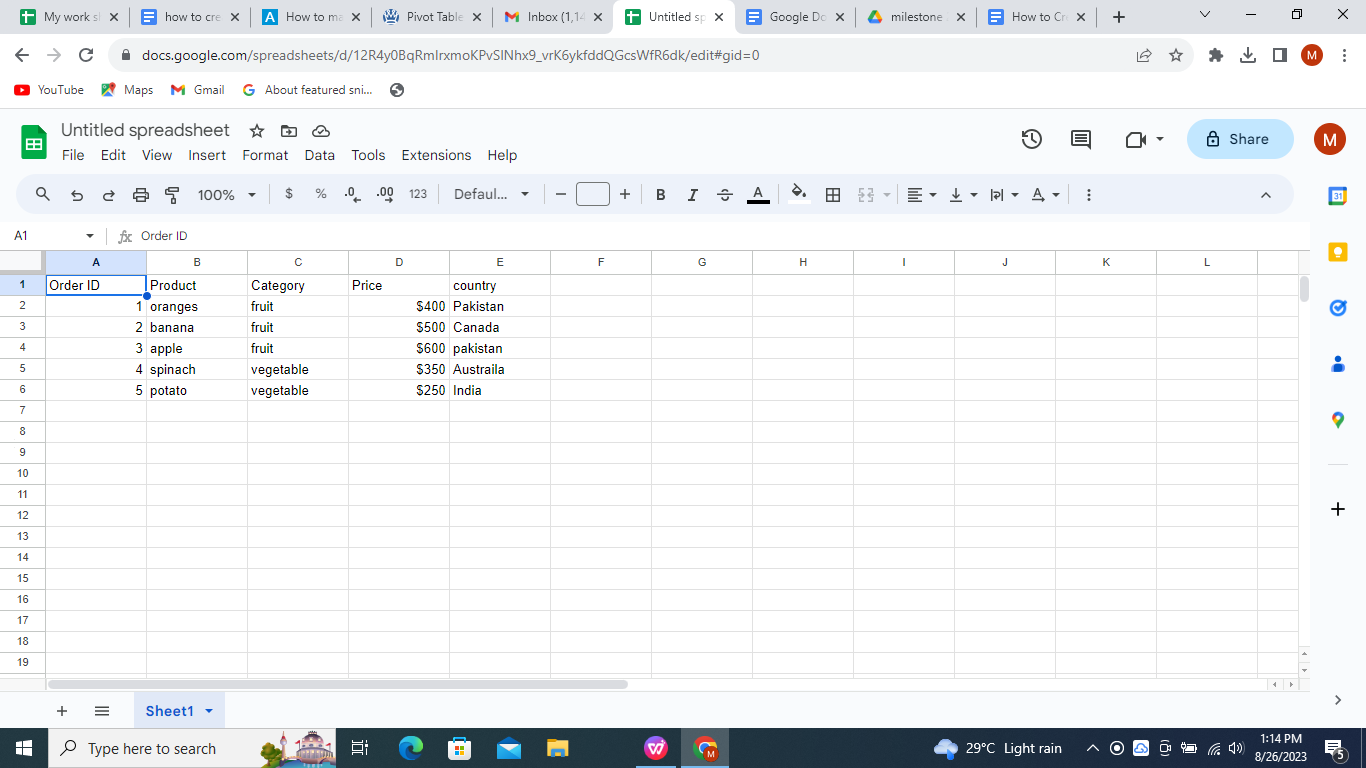
Step 1: Open your Excel Worksheet. Start by opening the Excel worksheet that contains the data you want to analyze. Make sure your data is organized with headers for each column.
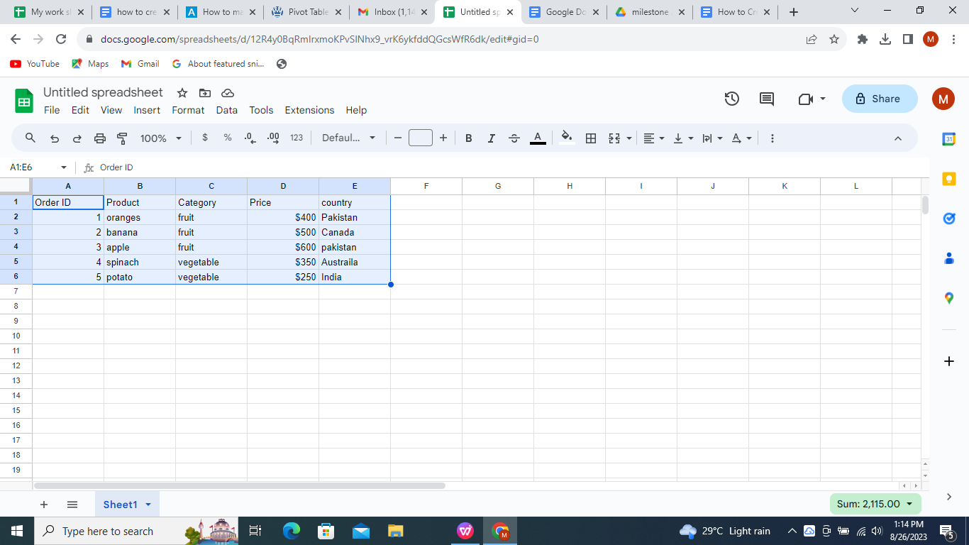
Step 2: Select Your Data. Click on any cell within your data range. This will help Excel understand the data you want to include in the Pivot Table.
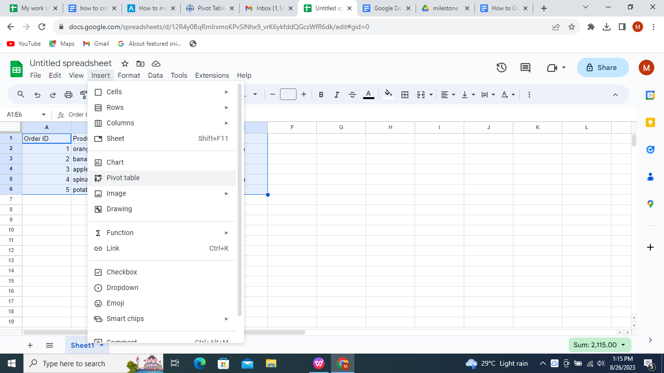
Step 3: Insert PivotTable. Navigate to the "Insert" tab in the Excel ribbon at the top. Click on the "PivotTable" button. A dialogue box will appear.
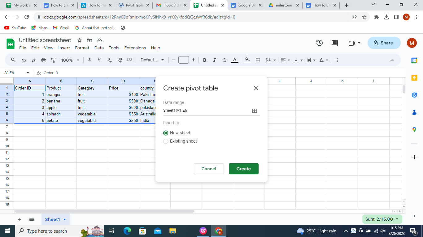
Step 4: Choose Data Range. In the dialogue box, make sure the correct data range is selected. You can also choose whether to place your PivotTable in a new or existing worksheet. Choose one of these options and click on the Create button.
Step 5: You'll see a new worksheet with a blank Pivot Table and a field list on the right. Drag or add the fields you want to analyze to the appropriate areas in the field list:
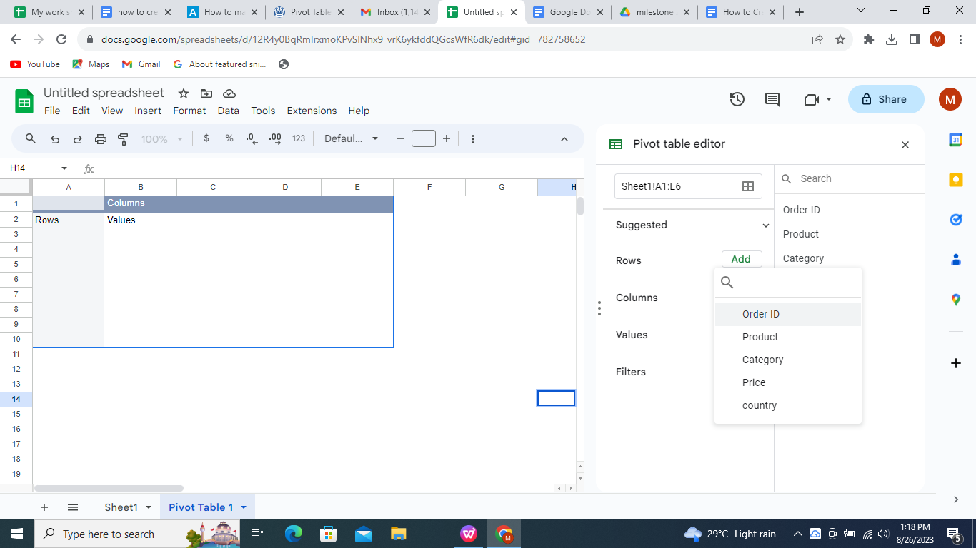
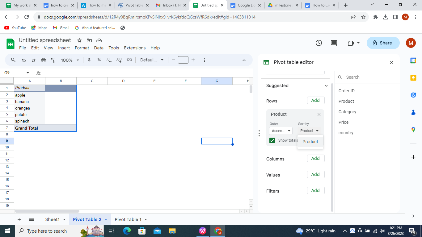
Step 6: Drag or add the fields to the "Rows" area to group data vertically.
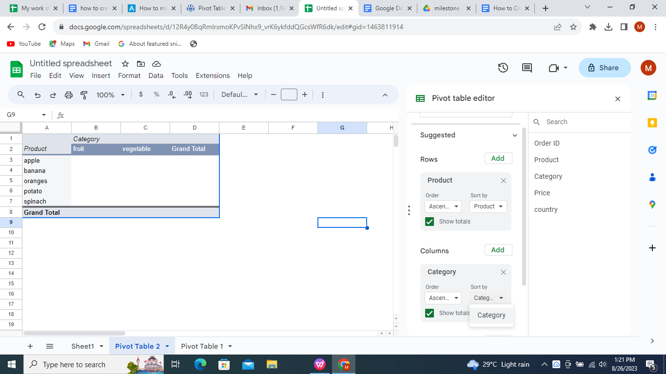
Step 7: Drag or add the fields to the "Columns" area to group data horizontally.
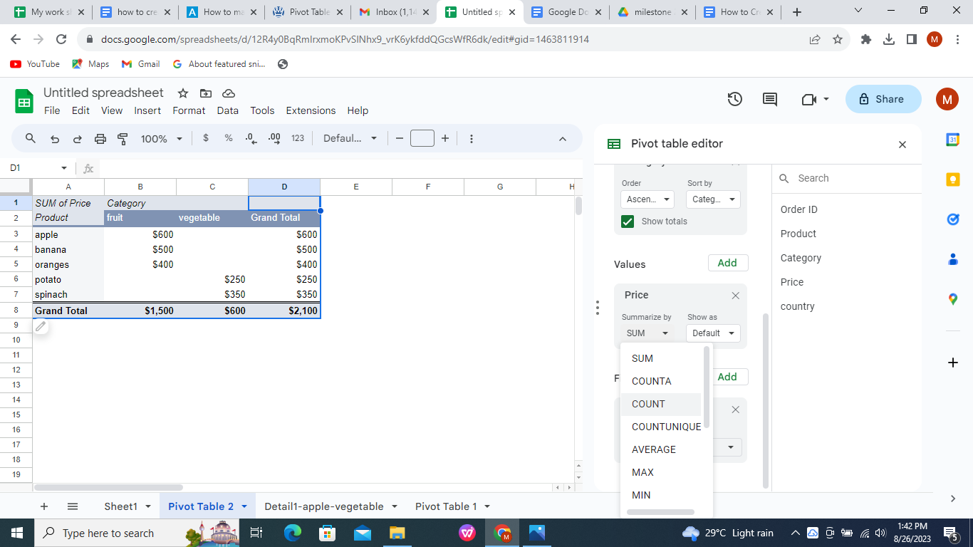
Step 8: Drag or add the fields to the "Values" area to perform calculations like sum, average, etc.
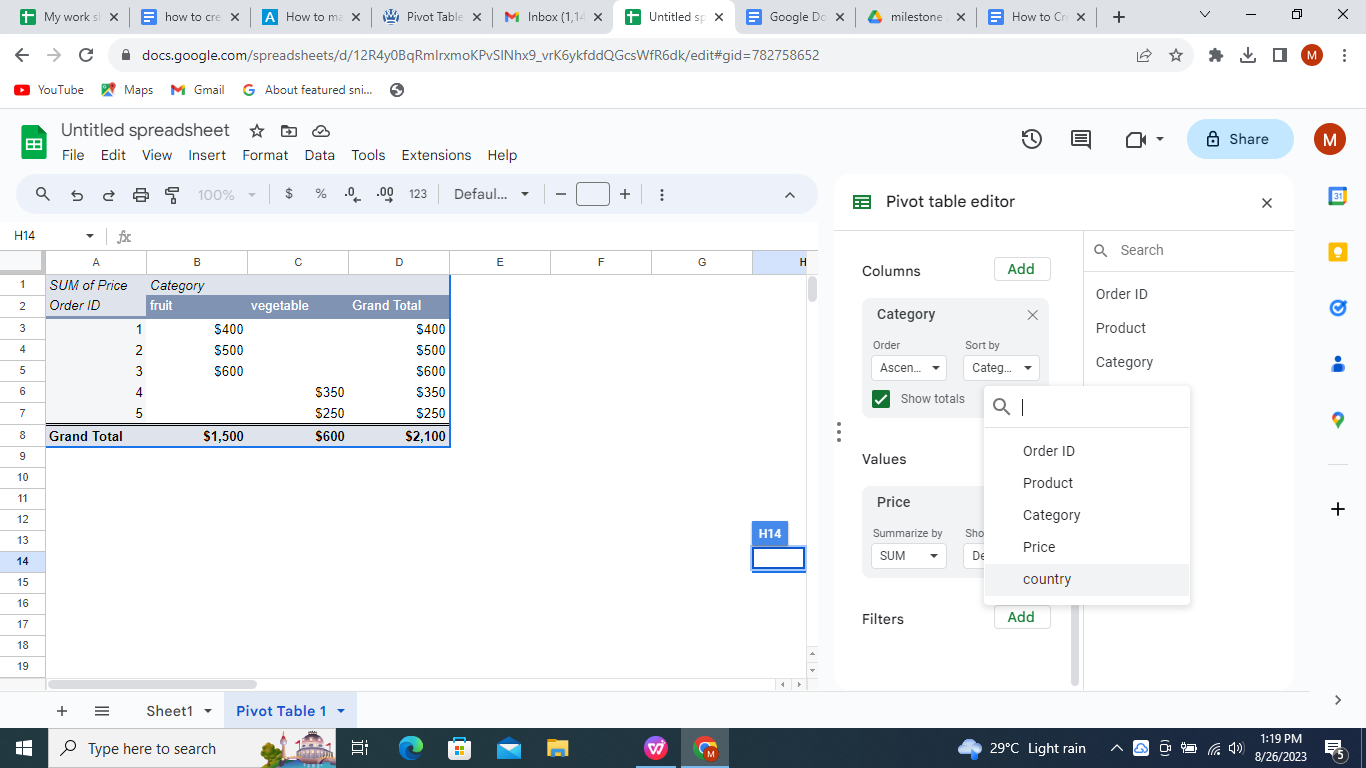
Step 9: You can customize Your pivot table. You can right-click on values in the Pivot Table to change how they're summarized. You can also use the "Value Field Settings" to specify the type of calculation you want to use.
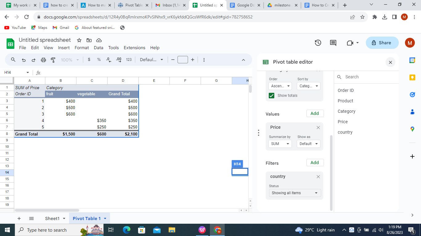
Step 10: Filter Your Data. You can filter your data by adding fields to the "Filters" area. This lets you focus on specific parts of your data in the Pivot Table.
Best Compatible Alternative to Microsoft Excel - WPS Office
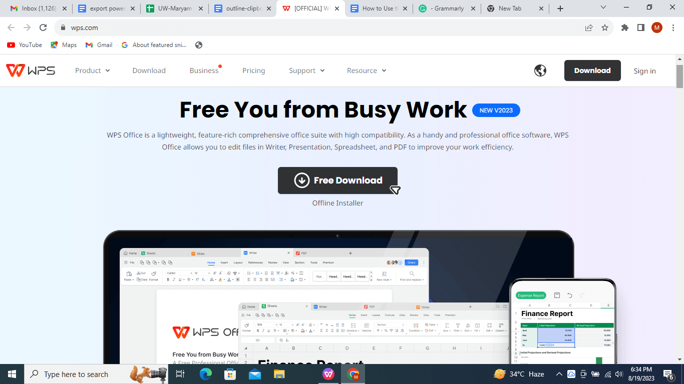
WPS Office is at the top of the list when finding the best compatible alternative to Microsoft Excel. Whether you're a seasoned data analyst or a student managing spreadsheets, WPS Office provides a seamless experience akin to Excel.

You can create a pivot table in a WPS Spreadsheet using similar methods as in Microsoft Excel. This ensures that if you're familiar with Excel's functionalities, transitioning to WPS Office is effortless.
You can employ the same techniques and principles to organize and analyze data efficiently.
Although Microsoft Excel and WPS Spreadsheet have the same features, their interfaces are identical. But we recommend you download the WPS spreadsheet for many compelling reasons.
Free Download: WPS Office is available as a free download, allowing you to access powerful spreadsheet capabilities without needing a premium subscription. This makes it an attractive option for individuals, students, and businesses seeking cost-effective solutions.
Compatibility: WPS Office offers many features that enhance your spreadsheet endeavors. From advanced data analysis tools to customizable charts and graphs, you'll find everything you need to extract insights from your data effectively.
User-friendly Interface: WPS Office has a similar interface to Microsoft Office that helps you to navigate the functions easily. It's easy to understand and easy to use.
Supports multiple Operating Systems: WPS Office, unlike Microsoft Office, supports multiple operating systems, including Windows, MacOS, Linux, Android, and iOS devices. WPS Office is reliable for all these platforms and ensures that you seamlessly complete your job without operating system limitations.
Rich template store: WPS office offers free and paid templates for Word, PPT, and Excel to help users save time and effort.
Requires small Storage: WPS Office is incredible for your memory. It provides all the features of Microsoft Office by consuming only 200MB of your device's memory. Isn't it awesome? So what are you waiting for?
Download WPS Office today and enjoy a 7-day free trial to unlock premium features!


FAQs About How to Create a Pivot Table in Excel
Q1: Can I customize the layout and appearance of the pivot table?
You can customize the appearance of the pivot table to make it look more attractive.
Follow these steps to customize your pivot table.
Step 1: Click on the PivotTable to see the PivotTable Tools option on the ribbon.
Step 2: Click the Design and the More button in the PivotTable Styles gallery to see all available styles and formats.
Step 3: Choose the style you like.
Step 4: If you find nothing interesting here, you can create your Design. Click on New PivotTable Styles at the bottom of the menu. Name your customized table, and you are all done!
Q2: What type of data is suitable for creating a pivot table?
You can use several types of data to create a pivot table. But, it's vital how you structure it.
You must structure your data skillfully to get more out of the Pivot table feature.
Here is a list of type of data that is suitable for creating a pivot table:
Numerical Data: It involves numbers, like sales, quantities, expenses, or ratings.
Categorical Data: Information with categories or labels, such as product names, items, customer segments, or geographic regions.
Time-Series Data: Data spanning time intervals, such as dates, hours, months, or years.
Transactional Data: Individual transactions, like customer orders or financial transactions.
Multi-Dimensional Data: Data with multiple dimensions, allowing for comparison across various aspects.
If you want to know how to create a pivot table in excel. Please read the above section.
Q3: How do you consolidate multiple worksheets into one Pivot Table?
Consolidating data from multiple worksheets into one Pivot Table can be highly valuable for comprehensive analysis. Follow this step-by-step guide to achieve this successfully:
Step 1: Create another worksheet where you want to place your consolidated Pivot Table.
Step 2: Navigate to the "Data" tab on the Excel ribbon.
Step 3: Click on the "Get Data" option. Depending on your Excel version, this could be "Get Data," "Get & Transform Data," or "Get External Data."
Step 4: In the drop-down menu that appears after clicking "Get Data," choose either the "Combine Queries" or "Consolidate" option. This might vary slightly based on your Excel version.
Step 5: If you choose "Combine Queries," select "Append Queries," then choose the worksheets you want to consolidate. If you choose "Consolidate," like the range of cells from each worksheet you want to include in the Pivot Table.
Step 6: Click "OK" or "Load" to bring the selected data from multiple worksheets into the new worksheet.
Step 7: Return to the new worksheet where you loaded the consolidated data. Select any cell within the data range. Then, go to the "Insert" tab on the Excel ribbon.
Step 8: Click on the "PivotTable" button. A dialogue box will appear.
Step 9: The date range will be pre-filled in the dialogue box. Make sure it covers all the consolidated data. You can place the Pivot Table in an existing or new worksheet.
Step 10: Like creating a regular PivotTable, drag the fields you want to analyze to the appropriate areas in the PivotTable Field List, such as rows, columns, and values.
Step 11: Your consolidated Pivot Table is now ready. Use it to analyze and explore data from multiple worksheets in a unified view.
Step 12: If the data in your source worksheets changes, right-click on the PivotTable and select "Refresh" to update the consolidated data.
Summary
Pivot table is a simple yet powerful data analysis tool to quickly summarize and manipulate large datasets, saving time and effort. This blog post provided a complete tutorial on how to create a pivot table in Excel to help you easily manage many data sheets.
While creating pivot tables in WPS Office Spreadsheet follows familiar methods used in Microsoft Excel, there are compelling reasons to choose WPS Office as your go-to spreadsheet solution.
The combination of free download, compatibility with Microsoft Office formats, rich features, and a user-friendly interface makes WPS Office a versatile and cost-efficient choice for your spreadsheet needs.

'%3e%3cpath%20d='M19.9911%204.11386V6.471H18.5894C18.0775%206.471%2017.7322%206.57814%2017.5536%206.79243C17.3751%207.00671%2017.2858%207.32814%2017.2858%207.75671V9.44421H19.9019L19.5536%2012.0871H17.2858V18.8639H14.5536V12.0871H12.2769V9.44421H14.5536V7.49779C14.5536%206.39064%2014.8632%205.53201%2015.4822%204.92189C16.1013%204.31177%2016.9257%204.00671%2017.9554%204.00671C18.8304%204.00671%2019.509%204.04243%2019.9911%204.11386Z'%20fill='%23333333'/%3e%3c/g%3e%3cdefs%3e%3cclipPath%20id='clip0_2938_8199'%3e%3crect%20width='16'%20height='16'%20fill='white'%20transform='translate(8%204.00671)'/%3e%3c/clipPath%3e%3c/defs%3e%3c/svg%3e)
'%3e%3cpath%20d='M17.5237%2010.7813L23.4811%204H22.0699L16.8949%209.88693L12.7648%204H8L14.2469%2012.9029L8%2020.0133H9.4112L14.8725%2013.7952L19.2352%2020.0133H24M9.92053%205.04213H12.0885L22.0688%2019.0224H19.9003'%20fill='%23333333'/%3e%3c/g%3e%3cdefs%3e%3cclipPath%20id='clip0_2938_8200'%3e%3crect%20width='16'%20height='16.0134'%20fill='white'%20transform='translate(8%204)'/%3e%3c/clipPath%3e%3c/defs%3e%3c/svg%3e)


