Free All-in-One Office Suite with PDF Editor
Edit Word, Excel, and PPT for FREE.
Read, edit, and convert PDFs with the powerful PDF toolkit.
Microsoft-like interface, easy to use.
Windows • MacOS • Linux • iOS • Android

How to combine two text cells in Excel
When you combine two cells in Excel, you're essentially just creating a copy of the data in one cell and then pasting it into the other cell. This is useful if you want to make sure that your data isn't accidentally duplicated.
For example, say you have a list of names and phone numbers for your employees. You want to track who's called in on each day so that you can give them their schedules. But when you look at the list of names, there are some duplicates i.e., someone has called in twice for the same day. So rather than deleting all the duplicates (which would take forever), you can combine these two cells and get rid of them all at once.
Tips that are provided in this article are compatible with versions 2010-2016 as well as the most recent 2021 version, MAC and online.
The CONCATENATE Function
The concatenate function in excel can be used to combine two or more text cells together. It is the simplest way to combine text cells. The steps are as follows:
1. Make sure you know the references of the text cells you wish to combine. For example, the text ‘Hello’ is in cell A1 and ‘World’ is in A2. The alphabets and letters describing the cells are on the horizontal and vertical axis of the spreadsheet respectively.

2. CONCATENATE function is easy to use. It is only required to type =CON in the target cell (where you need you text cells to be combined) and the drop-down menu of functions appears.

3. Select the CONCATENATE function by a double-click. A paraphrases is shown. The reference numbers of the cells you wish to combine are to be types inside. Make sure to separate both by a comma (,). The cells with be highlighted.

4. Press ‘Enter’ and you will receive your desired result.

5. This can be done for a large amount of cells. Make sure the order of the cells in the argument of the function (which is inside the parentheses) is as such your requirement. Version 2021 provides a clean display. For example, A1, B1,B2,B3,B4. The result is satisfactory.

6. Formulas can also be typed in the formula search box or in the main menu ‘formula section’.


The TEXTJOIN function in WPS Excel
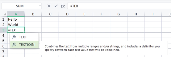
1. The TEXTJOIN function can be written as ‘=TEXTJOIN’ in the target cell, function search bar or main menu function generator.

2. This function also has a specific format for its argument as below. TRUE ignores empty cells.

3. Cells to be merged are written next. You can also select them by dragging across.

4. Press enter for result.

Combine text from different cells into a single cell using Ampersand (&)
‘&’ is a very useful tool in combining text cells. It is done in small, easy steps:
1. Select the target cell where you want to combine your text cells, for example A3. This was done in Version 2021 but it is also compatible with older versions, as well as 2016/2019/mac or online.

2. Type = and select the first cell you want to join. It will be selected and its reference will automatically be placed after ‘=’.

3. Next, type ’&’ and select the next cell you want to combine. It will also be selected and its reference will automatically be written in the target cell.

4. Press enter. The result is satisfactory.

Did you learn about how to combine two text cells in WPS Excel? You can follow WPS Academy to learn more features of Word Document, Excel Spreadsheets and PowerPoint Slides.
You can also download WPS Office to edit the word documents, excel, PowerPoint for free of cost. Download now! And get an easy and enjoyable working experience.
Also Read:
- 1. How to split text in only two rows in excel
- 2. How to Multiply Two Cells in Excel Spreadsheet Using WPS Office:A Step-by-Step Guide
- 3. How to extract text between two characters in Excel
- 4. How to combine only two text cells in Excel
- 5. How to Compare the Values of Two Cells in Excel
- 6. How to combine text from two cells in Excel (3 Simplest Methods)
