
'%3e%3cpath%20d='M8%200C12.4183%200%2016%203.58172%2016%208C16%2012.4183%2012.4183%2016%208%2016C3.58172%2016%200%2012.4183%200%208C0%203.58172%203.58172%200%208%200ZM11.6162%204.38379C11.2257%203.99337%2010.5927%203.99338%2010.2021%204.38379L8%206.58594L5.79785%204.38379C5.40732%203.99334%204.77429%203.99329%204.38379%204.38379C3.99331%204.77429%203.99335%205.40733%204.38379%205.79785L6.58594%208L4.38379%2010.2021C3.99348%2010.5927%203.99341%2011.2257%204.38379%2011.6162C4.77426%2012.0066%205.40734%2012.0065%205.79785%2011.6162L8%209.41406L10.2021%2011.6162C10.5927%2012.0066%2011.2257%2012.0067%2011.6162%2011.6162C12.0067%2011.2257%2012.0066%2010.5927%2011.6162%2010.2021L9.41406%208L11.6162%205.79785C12.0066%205.40735%2012.0066%204.77429%2011.6162%204.38379Z'%20fill='%23080E17'%20fill-opacity='0.46'/%3e%3c/g%3e%3cdefs%3e%3cclipPath%20id='clip0_3761_713'%3e%3crect%20width='16'%20height='16'%20fill='white'/%3e%3c/clipPath%3e%3c/defs%3e%3c/svg%3e)


'%3e%3cpath%20fill-rule='evenodd'%20clip-rule='evenodd'%20d='M21.4999%2010.9993C21.4999%205.20009%2016.7986%200.498901%2010.9993%200.498901C5.19994%200.498901%200.498657%205.20009%200.498657%2010.9993C0.498657%2016.2404%204.33858%2020.5844%209.35855%2021.3722V14.0346H6.69238V10.9993H9.35855V8.68594C9.35855%206.05427%2010.9262%204.60062%2013.3248%204.60062C14.4736%204.60062%2015.6753%204.80571%2015.6753%204.80571V7.38979H14.3512C13.0468%207.38979%2012.64%208.19921%2012.64%209.0296V10.9993H15.5523L15.0867%2014.0346H12.64V21.3722C17.66%2020.5844%2021.4999%2016.2404%2021.4999%2010.9993Z'%20fill='%231568EA'/%3e%3c/g%3e%3c/svg%3e)


Navigating the world of subtraction formulas in Google Sheets can be challenging. In this guide, we'll simplify the process, sharing insights and tips along the way. Join us as we explore the nuances of subtraction, making spreadsheet calculations a breeze.
What Is Subtraction Formula in Google Sheets

In Google Sheets, the subtraction formula is primarily executed through the use of the MINUS function. The MINUS function allows users to subtract numbers or cells, facilitating accurate numerical calculations within a spreadsheet. Its syntax is straightforward: you input the numbers or cell references you want to subtract, separated by the minus sign ("-"). For example, "=MINUS(A2, B2)" subtracts the value in cell B2 from the value in cell A2.
Syntax:
=MINUS(number1, number2)
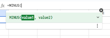
Here, "number1" is the minuend (the number you want to subtract from), and "number2" is the subtrahend (the number you want to subtract). The result is the numerical difference between the two.
Usage Example: Consider a scenario where you have values in cells A2 and B2, and you want to find the difference. The formula would look like this:
=MINUS(A2, B2)
Easiest Way to Subtract in Google Sheets Without Formulas
The - (minus) operator provides a simple and direct method for subtraction in Google Sheets, ideal for quick calculations without intricate formulas. Follow this step-by-step guide to efficiently subtract values:
Step 1: Open Your Google Sheet Ensure you are in the Google Sheet containing the values you want to subtract.

Step 2: Select the Target Cell Click on the cell where you want the result of the subtraction to appear.
Step 3: Input the Subtraction Operation Type the subtraction operation using the - (minus) operator. For example, to subtract the value in cell B2 from A2, type:
=A2 - B2
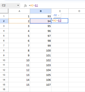
Step 4: Press Enter Hit the Enter key to execute the operation and view the result in the selected cell.
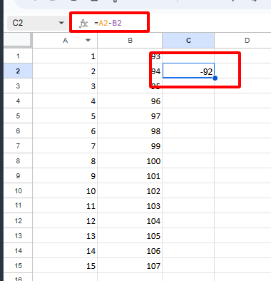
This straightforward method allows you to perform basic subtractions without the need for complex formulas. By simply using the minus (-) operator and cell references, you can quickly determine the difference between any two values in your Google Sheet.
How to Subtract in Google Sheets Using Formulas
Subtracting values in Google Sheets is a fundamental operation that can be accomplished using formulas. Formulas provide greater flexibility and control over the subtraction process, enabling you to perform more complex calculations.
To subtract multiple numbers in Google Sheets
To subtract multiple numbers in Google Sheets, you can use the minus (-) operator within a formula. Here's a step-by-step guide:
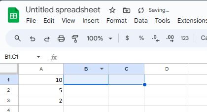
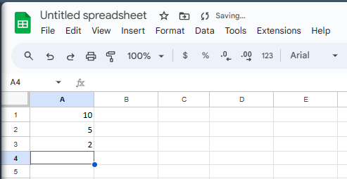
Step 1: Enter the Numbers
Begin by entering the numbers you want to subtract in separate cells. For instance, if you want to subtract 10, 5, and 2, enter them in cells A1, A2, and A3, respectively.
Step 2: Select the Destination Cell
Click on the cell where you want the subtraction result to appear. In this example, select cell A4.
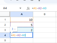
Step 3: Type the Formula
Start by typing the equal sign (=) in the selected cell (A4). Then, type the minus (-) operator followed by the cell references containing the values you want to subtract, separated by commas. In this case, type:
=A1-A2-A3
This formula instructs Google Sheets to subtract the value in cell A2 from the value in cell A1, and then subtract the result from the value in cell A3.
Step 4: Press Enter
Once you've entered the complete formula, press the Enter key on your keyboard. Google Sheets will automatically calculate the difference and display the result in cell A4.
To subtract multiple cell references in Google Sheets
You can also subtract values from multiple cell references using the MINUS function in Google Sheets. Here's a step-by-step guide:
Step 1: Enter the Values
Enter the values you want to subtract in separate cells. For instance, if you want to subtract the values in cells A1 to A3, enter them in their respective cells.
Step 2: Select the Destination Cell
Click on the cell where you want the subtraction result to appear. In this example, select cell A4.
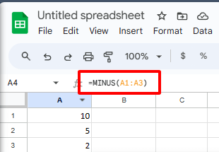
Step 3: Type the MINUS Function
Start by typing the equal sign (=) in the selected cell (A4). Then, type the MINUS function followed by the range of cells containing the values you want to subtract. In this case, type:
=MINUS(A1:A3)
This formula instructs Google Sheets to subtract the values in the range A1:A3 from each other and display the result in cell A4.
Step 4: Press Enter
Once you've entered the complete formula, press the Enter key on your keyboard. Google Sheets will automatically calculate the difference and display the result in cell A4.
By utilizing formulas, you can subtract multiple numbers and cell references in Google Sheets, enabling you to perform more complex calculations and analyze data effectively.
[Extended] How to Add in Google Sheets Using Formulas
n this extended section, we explore the SUM function in Google Sheets—a versatile tool for adding numbers efficiently. Below is a brief introduction to the SUM function and a step-by-step guide for optimal understanding:
Introduction to SUM Function:
The SUM function in Google Sheets is designed to add up a range of numbers or cell references, providing a total sum. Its syntax is simple and effective:
=SUM(number1, number2, ...)
Here, "number1," "number2," and so on represent the values you want to add together.
Step-by-Step Guide:
Step 1: Open Your Google Sheet Access the Google Sheet containing the numbers or cell references you want to add.
Step 2: Select the Target Cell Click on the cell where you want the sum to appear.
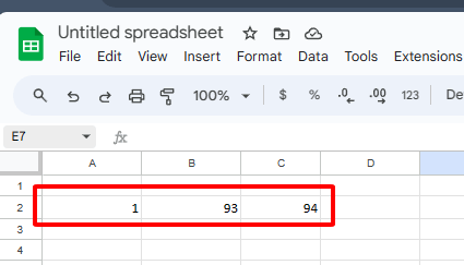
Step 3: Input the SUM Formula Type the SUM formula, including the cell references or numbers you want to add. For instance, to add the values in cells A2, B2, and C2, type:
=SUM(A2, B2, C2)
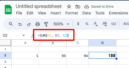
Step 4: Press Enter Press the Enter key to execute the formula and showcase the total sum in the selected cell.
By mastering the SUM function, users can efficiently add numbers or cell references in Google Sheets, facilitating accurate and streamlined calculations within their spreadsheets.
Best Free Alternative to Google Sheets - WPS Spreadsheet

For users seeking a robust alternative to Google Sheets, WPS Spreadsheet from WPS Office stands out with a range of features that enhance productivity and efficiency. Here's an overview, emphasizing its key attributes:
Free Download and Free to Use: WPS Spreadsheet offers a compelling advantage with its free-to-use model. Users can download and access the software without any cost, making it an economical choice for individuals and businesses alike.
File Compatibility: WPS Spreadsheet works smoothly with both Microsoft Excel and WPS Spreadsheet files. This means you can switch between platforms without worrying about data or formatting issues.
Free PDF Editing Tools: In addition to spreadsheet functionalities, WPS Office provides users with free PDF editing tools. This versatile feature allows for easy manipulation of PDF documents, enhancing the overall document management experience within the WPS ecosystem.
Delicate Office Templates: WPS Spreadsheet comes with a built-in Template Library offering professional office templates. Downloading and using these templates saves time and effort in creating polished and well-organized documents
WPS AI Integration: Thanks to WPS AI, WPS Office becomes smarter. It analyzes documents, helps with formatting, and gives intelligent content recommendations, streamlining the document creation process for improved productivity

In conclusion, WPS Spreadsheet emerges as a compelling free alternative to Google Sheets, offering a suite of features that cater to various user needs, from file compatibility to advanced AI-driven enhancements, making it a worthy choice for those looking to diversify their spreadsheet software options.
FAQs
How to make numbers negative in Google Sheets?
To make a number negative in Google Sheets, simply add a minus sign ("-") before the number. For instance, typing =-A1 makes the value in cell A1 negative.
What is the most common function in Google Sheets?
The most common function in Google Sheets is the SUM function (=SUM()). It adds up a range of numbers or cell values. For example, =SUM(A1:A10) calculates the sum of values in cells A1 through A10.
How can I quickly sum a range of numbers in Google Sheets?
To swiftly calculate the sum of a range in Google Sheets, use the SUM function. Simply enter "=SUM(" followed by the range of cells you want to add, and close with a parenthesis. For example, to sum the values in cells A1 to A10, type "=SUM(A1:A10)" in the desired cell. This formula automates the addition process, providing an efficient way to obtain the total sum of selected numbers in your spreadsheet.
Summary
This guide helps you easily use subtraction formulas in Google Sheets, providing step-by-step instructions for both basic and advanced techniques. Learn about the MINUS function, the - (minus) operator, and how to subtract multiple cells or entire columns. The article also introduces the SUM function for addition. Plus, discover WPS Office as a robust alternative with features like file compatibility and free PDF editing tools. Whether you're a beginner or looking for advanced spreadsheet solutions, this guide ensures accuracy and efficiency in your calculations.

'%3e%3cpath%20d='M19.9911%204.11386V6.471H18.5894C18.0775%206.471%2017.7322%206.57814%2017.5536%206.79243C17.3751%207.00671%2017.2858%207.32814%2017.2858%207.75671V9.44421H19.9019L19.5536%2012.0871H17.2858V18.8639H14.5536V12.0871H12.2769V9.44421H14.5536V7.49779C14.5536%206.39064%2014.8632%205.53201%2015.4822%204.92189C16.1013%204.31177%2016.9257%204.00671%2017.9554%204.00671C18.8304%204.00671%2019.509%204.04243%2019.9911%204.11386Z'%20fill='%23333333'/%3e%3c/g%3e%3cdefs%3e%3cclipPath%20id='clip0_2938_8199'%3e%3crect%20width='16'%20height='16'%20fill='white'%20transform='translate(8%204.00671)'/%3e%3c/clipPath%3e%3c/defs%3e%3c/svg%3e)
'%3e%3cpath%20d='M17.5237%2010.7813L23.4811%204H22.0699L16.8949%209.88693L12.7648%204H8L14.2469%2012.9029L8%2020.0133H9.4112L14.8725%2013.7952L19.2352%2020.0133H24M9.92053%205.04213H12.0885L22.0688%2019.0224H19.9003'%20fill='%23333333'/%3e%3c/g%3e%3cdefs%3e%3cclipPath%20id='clip0_2938_8200'%3e%3crect%20width='16'%20height='16.0134'%20fill='white'%20transform='translate(8%204)'/%3e%3c/clipPath%3e%3c/defs%3e%3c/svg%3e)


