
'%3e%3cpath%20d='M8%200C12.4183%200%2016%203.58172%2016%208C16%2012.4183%2012.4183%2016%208%2016C3.58172%2016%200%2012.4183%200%208C0%203.58172%203.58172%200%208%200ZM11.6162%204.38379C11.2257%203.99337%2010.5927%203.99338%2010.2021%204.38379L8%206.58594L5.79785%204.38379C5.40732%203.99334%204.77429%203.99329%204.38379%204.38379C3.99331%204.77429%203.99335%205.40733%204.38379%205.79785L6.58594%208L4.38379%2010.2021C3.99348%2010.5927%203.99341%2011.2257%204.38379%2011.6162C4.77426%2012.0066%205.40734%2012.0065%205.79785%2011.6162L8%209.41406L10.2021%2011.6162C10.5927%2012.0066%2011.2257%2012.0067%2011.6162%2011.6162C12.0067%2011.2257%2012.0066%2010.5927%2011.6162%2010.2021L9.41406%208L11.6162%205.79785C12.0066%205.40735%2012.0066%204.77429%2011.6162%204.38379Z'%20fill='%23080E17'%20fill-opacity='0.46'/%3e%3c/g%3e%3cdefs%3e%3cclipPath%20id='clip0_3761_713'%3e%3crect%20width='16'%20height='16'%20fill='white'/%3e%3c/clipPath%3e%3c/defs%3e%3c/svg%3e)


'%3e%3cpath%20fill-rule='evenodd'%20clip-rule='evenodd'%20d='M21.4999%2010.9993C21.4999%205.20009%2016.7986%200.498901%2010.9993%200.498901C5.19994%200.498901%200.498657%205.20009%200.498657%2010.9993C0.498657%2016.2404%204.33858%2020.5844%209.35855%2021.3722V14.0346H6.69238V10.9993H9.35855V8.68594C9.35855%206.05427%2010.9262%204.60062%2013.3248%204.60062C14.4736%204.60062%2015.6753%204.80571%2015.6753%204.80571V7.38979H14.3512C13.0468%207.38979%2012.64%208.19921%2012.64%209.0296V10.9993H15.5523L15.0867%2014.0346H12.64V21.3722C17.66%2020.5844%2021.4999%2016.2404%2021.4999%2010.9993Z'%20fill='%231568EA'/%3e%3c/g%3e%3c/svg%3e)


When it comes to analyzing data, P-value is an essential concept that helps to determine the significance of the results obtained from regression or correlation analysis. However, calculating P-value manually can be a daunting task, with a high probability of errors. That's where spreadsheet tools come in handy, allowing you to calculate P-value with a few clicks. If you're wondering how to do that, keep reading, as we'll introduce you to three easy ways to calculate P-value using Excel's built-in functions and formulas.
What is the P-Value?
The P-value is a statistical measure used to determine the probability of obtaining a result equal to or more extreme than the observed result, assuming the null hypothesis is true. It is often used in hypothesis testing to determine whether there is enough evidence to reject the null hypothesis and accept the alternative hypothesis. A P-value of less than 0.05 (or 0.01) is typically considered statistically significant and indicates that there is strong evidence against the null hypothesis.
Two Formulas to Calculate P-value
TDIST and TTEST are two excel formulas used to calculate P-value. Here's a brief overview of each:
TDIST:
TDIST calculates the one-tailed probability of the Student's t-distribution. It is commonly used in hypothesis testing to determine whether a sample mean is significantly different from a known or hypothesized population mean. The formula takes three arguments: x (the test value), degrees of freedom, and tails (the number of tails in the distribution).
Syntax: TDIST(x, degrees_freedom, tails)
TTEST:
TTEST is used to calculate the probability that two samples are from the same population, based on the assumption that the samples are normally distributed and have equal variances. The formula takes four arguments: array1 (the first data set), array2 (the second data set), tails (the number of tails in the distribution), and type (specifies the type of t-test to perform).
Syntax: TTEST(array1, array2, tails, type)
Calculate P-value in Excel with TDIST Function
When conducting statistical hypothesis tests, P-value is a crucial indicator of the probability that the results obtained are due to chance. Excel offers various methods to calculate P-value, but one of the most common is the TDIST function. In this article, we will discuss three ways to calculate P-value using the TDIST function in Excel.
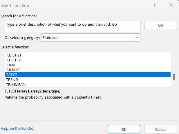
Method 1: Using Insert function button
1. Select the cell where you want to calculate the P-value.
2. Click on the "fx" button next to the formula bar to open the Insert Function dialog box.

3. In the search bar, type "TDIST" and select it from the list of functions.
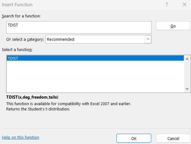
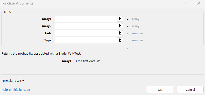
4. Enter the appropriate values for the arguments in the Function Arguments dialog box.
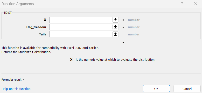
5. Click OK to close the dialog box and calculate the P-value.
Method 2: Using Statistical formula section
1. Select the cell where you want to calculate the P-value.
2. Click on the "Formulas" tab in the ribbon.

3. In the "More Functions" dropdown menu, select "Statistical."

4. Select "TDIST" from the list of functions.
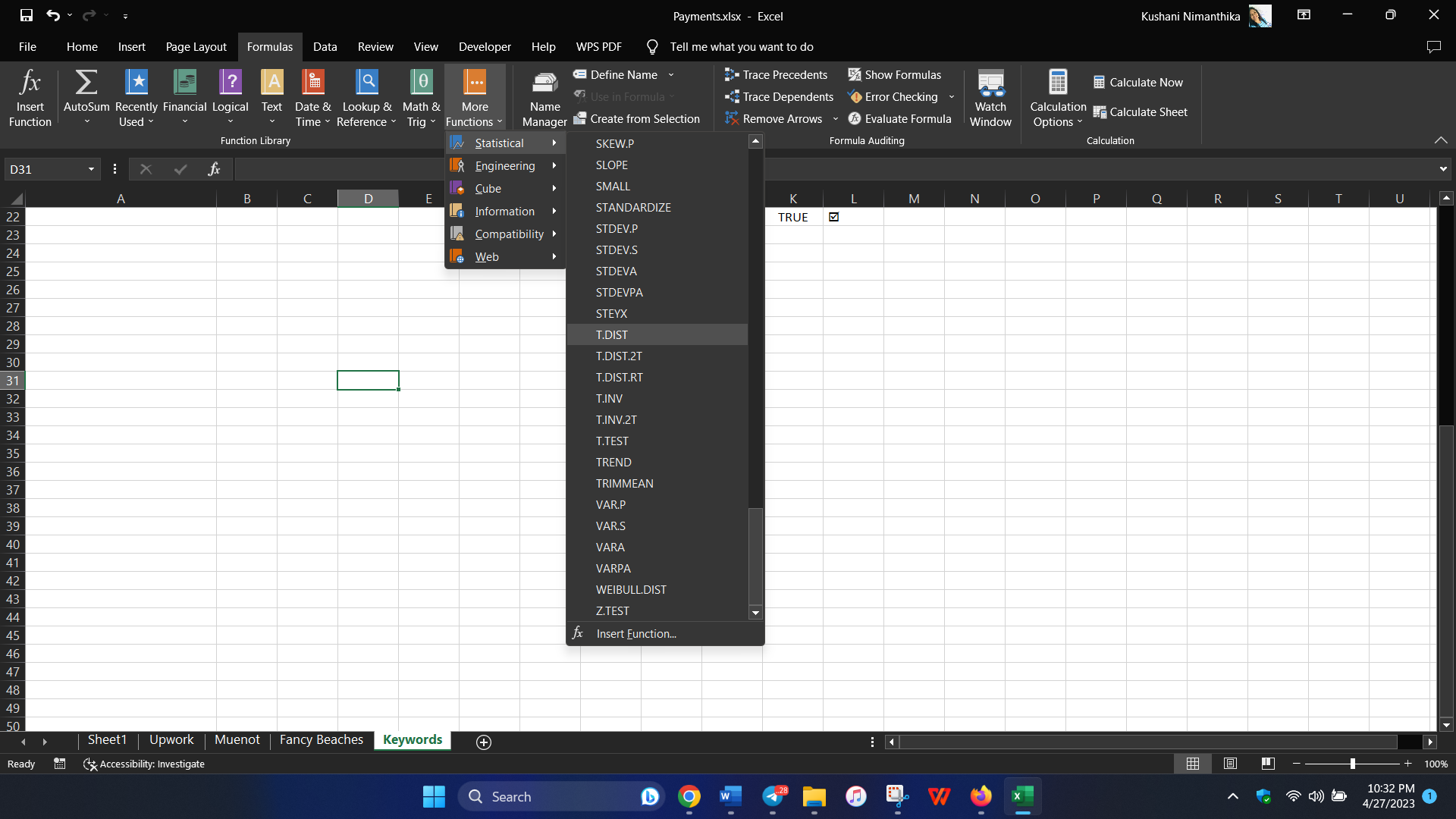
5. Enter the appropriate values for the arguments in the Function Arguments dialog box.
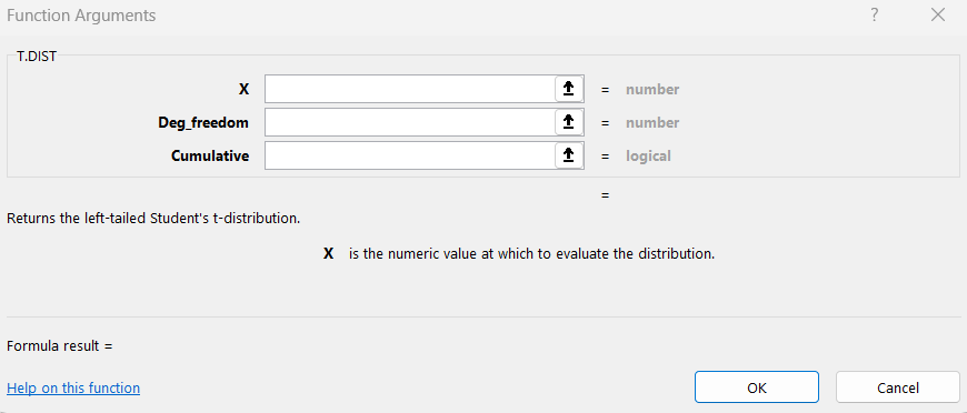
6. Click OK to close the dialog box and calculate the P-value.
Method 3: Manually entering P-value Formula
Select the cell where you want to calculate the P-value.
Enter the formula "=TDIST(x, degrees of freedom, tails)" in the formula bar.
Replace "x" with the test statistic value, "degrees of freedom" with the appropriate degrees of freedom value, and "tails" with the number of tails in the distribution.
Press Enter to calculate the P-value.
Calculate P-value in Excel with TTEST Function
It should be noted that while the methods of applying TDIST and TTEST functions in Excel are similar, they require different arguments. Here are three methods for calculating P-value using the TTEST function in Excel:
Method 1: Using the Insert Function button
1. Select the cell where you want to place the P-value result.
2. Click on the "fx" button next to the formula bar.
3. Search for the TTEST function and select it.
4. Enter the arguments for the function, including the data arrays and the type of test you want to perform.
5. Click "OK" to see the result.
Method 2: Using the Statistical formula section
1. Select the cell where you want to place the P-value result.
2. Go to the "Formulas" tab in the ribbon.
3. Click on "More Functions" and select "Statistical".
4. Choose the TTEST function.
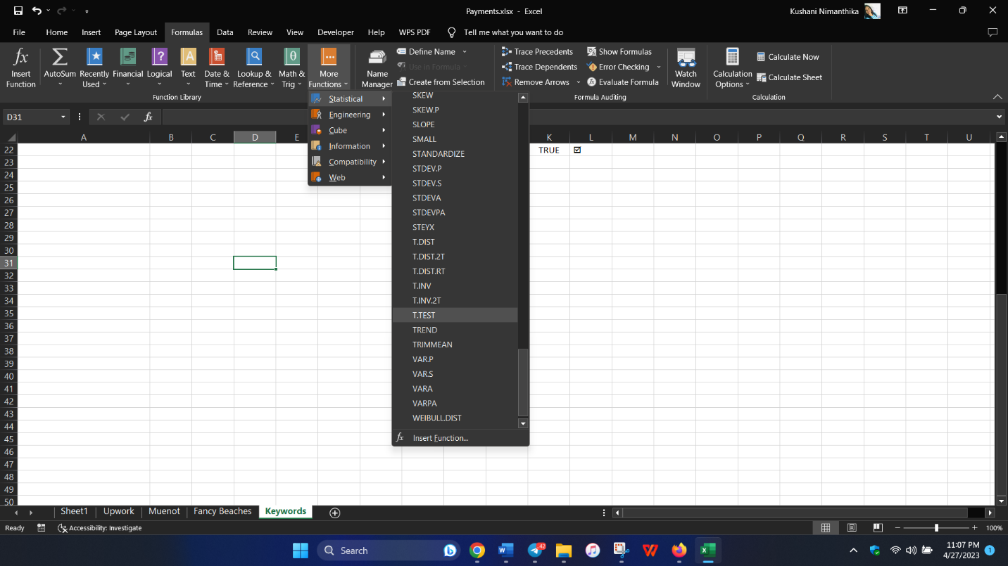
5. Enter the arguments for the function and click "OK" to see the result.
Method 3: Manually entering the P-value formula
Use the formula =T.TEST(data_array1, data_array2, tails, type) in the cell where you want to place the P-value result.
Enter the data arrays and specify the number of tails and the type of test you want to perform.
Press "Enter" to see the result.
Calculate P-value in Excel with Analysis Toolpak
When it comes to hypothesis testing, calculating P-values is an essential step to determine the significance of your results. In Excel, there are several ways to calculate P-values, including using built-in formulas such as TDIST and TTEST. However, another powerful tool to help you with this task is the Analysis Toolpak add-in, which can be installed to get access to advanced data analysis functions. In this section, we will show you how to use the Analysis Toolpak to calculate P-value in Excel.
Installing Analysis Toolpak
Open Excel and click on File
Click on Options, and then select Add-ins
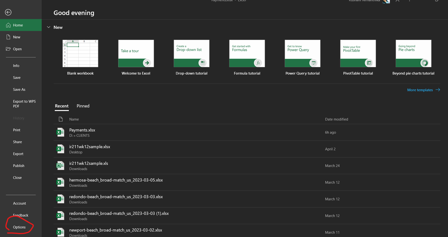
Select Excel Add-ins, and then click on the Go button
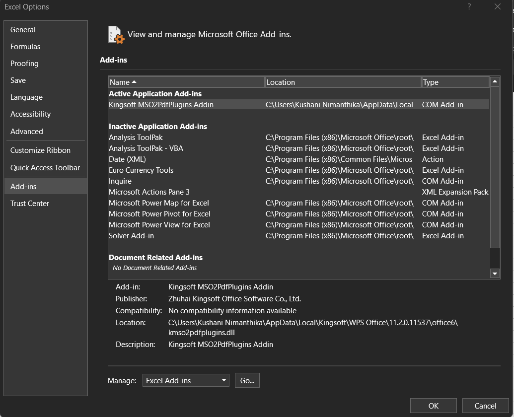
Check the Analysis Toolpak box, and then click on OK
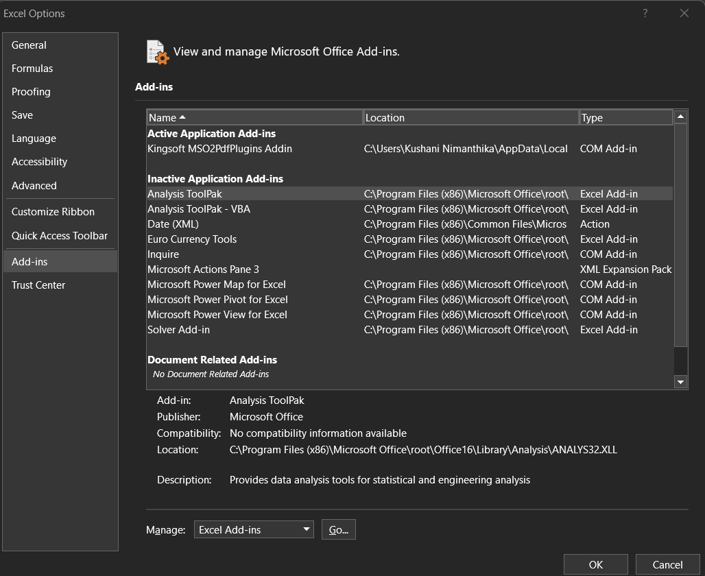
Wait for the tool to install
Using Analysis Toolpak to Calculate P-Value
Enter your data in a spreadsheet
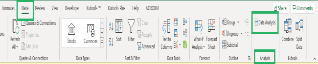
Click on the Data tab, and then select Data Analysis from the Analysis group
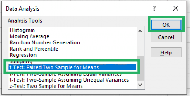
Select t-Test: Paired Two Sample for Means, and then click on OK
Enter the Input Range for Variable 1 and Variable 2
Set the Hypothesized Mean Difference to 0
Select a level of significance for your test
Select the Output Range where you want the results to appear
Click on OK to run the test
Using the Analysis Toolpak add-in in Excel can help you perform advanced data analysis functions, including calculating P-values. With this powerful tool, you can easily analyze your data and determine the significance of your results.
Possible Errors When Calculating in Excel
When calculating P-value in Excel, there are several possible errors that you may encounter. Here are some of the most common ones:
#DIV/0! error: This error occurs when you try to divide a number by zero or a blank cell. To fix this error, you can either change the denominator to a non-zero number or enter a value in the blank cell.
#VALUE! error: This error occurs when Excel is unable to recognize a formula or function. This could be because of a typo or incorrect syntax. Double-check your formula or function to ensure it is entered correctly.
#NAME? error: This error occurs when Excel is unable to recognize a name in a formula or function. This could be because of a typo or incorrect syntax. Double-check the spelling of the name and ensure it is entered correctly.
#REF! error: This error occurs when a formula or function refers to a cell or range of cells that no longer exists. This could be because the cell or range was deleted or moved. To fix this error, update the formula or function to reference the correct cell or range.
#NUM! error: This error occurs when a formula or function returns a numeric value that is not valid. This could be because of a mathematical error, such as dividing by a very large or very small number. Double-check your formula or function to ensure it is correct.
By being aware of these errors, you can avoid them and ensure accurate calculations in Excel.
FAQs about Calculate P-Value in Excel
What are the new functions that can replace the TDIST Functions?
The new functions that can replace the TDIST function in Excel are the T.DIST.2T function and T.DIST.RT function. These functions are more versatile and can handle two-tailed and right-tailed distributions.
How to analyse the P-value?
To analyze the P-value, you need to compare it with the level of significance or alpha value. If the P-value is less than the alpha value, then you reject the null hypothesis and accept the alternative hypothesis. If the P-value is greater than the alpha value, then you fail to reject the null hypothesis.
What are the most-used calculation functions in Excel?
The most-used calculation functions in Excel include SUM, AVERAGE, MAX, MIN, COUNT, COUNTIF, SUMIF, IF, AND, OR, and VLOOKUP, among others.

'%3e%3cpath%20d='M19.9911%204.11386V6.471H18.5894C18.0775%206.471%2017.7322%206.57814%2017.5536%206.79243C17.3751%207.00671%2017.2858%207.32814%2017.2858%207.75671V9.44421H19.9019L19.5536%2012.0871H17.2858V18.8639H14.5536V12.0871H12.2769V9.44421H14.5536V7.49779C14.5536%206.39064%2014.8632%205.53201%2015.4822%204.92189C16.1013%204.31177%2016.9257%204.00671%2017.9554%204.00671C18.8304%204.00671%2019.509%204.04243%2019.9911%204.11386Z'%20fill='%23333333'/%3e%3c/g%3e%3cdefs%3e%3cclipPath%20id='clip0_2938_8199'%3e%3crect%20width='16'%20height='16'%20fill='white'%20transform='translate(8%204.00671)'/%3e%3c/clipPath%3e%3c/defs%3e%3c/svg%3e)
'%3e%3cpath%20d='M17.5237%2010.7813L23.4811%204H22.0699L16.8949%209.88693L12.7648%204H8L14.2469%2012.9029L8%2020.0133H9.4112L14.8725%2013.7952L19.2352%2020.0133H24M9.92053%205.04213H12.0885L22.0688%2019.0224H19.9003'%20fill='%23333333'/%3e%3c/g%3e%3cdefs%3e%3cclipPath%20id='clip0_2938_8200'%3e%3crect%20width='16'%20height='16.0134'%20fill='white'%20transform='translate(8%204)'/%3e%3c/clipPath%3e%3c/defs%3e%3c/svg%3e)


