
'%3e%3cpath%20d='M8%200C12.4183%200%2016%203.58172%2016%208C16%2012.4183%2012.4183%2016%208%2016C3.58172%2016%200%2012.4183%200%208C0%203.58172%203.58172%200%208%200ZM11.6162%204.38379C11.2257%203.99337%2010.5927%203.99338%2010.2021%204.38379L8%206.58594L5.79785%204.38379C5.40732%203.99334%204.77429%203.99329%204.38379%204.38379C3.99331%204.77429%203.99335%205.40733%204.38379%205.79785L6.58594%208L4.38379%2010.2021C3.99348%2010.5927%203.99341%2011.2257%204.38379%2011.6162C4.77426%2012.0066%205.40734%2012.0065%205.79785%2011.6162L8%209.41406L10.2021%2011.6162C10.5927%2012.0066%2011.2257%2012.0067%2011.6162%2011.6162C12.0067%2011.2257%2012.0066%2010.5927%2011.6162%2010.2021L9.41406%208L11.6162%205.79785C12.0066%205.40735%2012.0066%204.77429%2011.6162%204.38379Z'%20fill='%23080E17'%20fill-opacity='0.46'/%3e%3c/g%3e%3cdefs%3e%3cclipPath%20id='clip0_3761_713'%3e%3crect%20width='16'%20height='16'%20fill='white'/%3e%3c/clipPath%3e%3c/defs%3e%3c/svg%3e)


'%3e%3cpath%20fill-rule='evenodd'%20clip-rule='evenodd'%20d='M21.4999%2010.9993C21.4999%205.20009%2016.7986%200.498901%2010.9993%200.498901C5.19994%200.498901%200.498657%205.20009%200.498657%2010.9993C0.498657%2016.2404%204.33858%2020.5844%209.35855%2021.3722V14.0346H6.69238V10.9993H9.35855V8.68594C9.35855%206.05427%2010.9262%204.60062%2013.3248%204.60062C14.4736%204.60062%2015.6753%204.80571%2015.6753%204.80571V7.38979H14.3512C13.0468%207.38979%2012.64%208.19921%2012.64%209.0296V10.9993H15.5523L15.0867%2014.0346H12.64V21.3722C17.66%2020.5844%2021.4999%2016.2404%2021.4999%2010.9993Z'%20fill='%231568EA'/%3e%3c/g%3e%3c/svg%3e)


If you want to unlock the full potential of Pivot Charts in Excel and effortlessly create them, this article is here to guide you every step of the way. By following the instructions provided, you'll not only learn how to create Pivot Charts but also understand the numerous benefits they offer. Pivot Charts enable you to summarize, analyze, and visualize data with ease, allowing you to gain valuable insights from your information. With their interactive and dynamic nature, Pivot Charts provide a seamless data exploration experience, empowering you to make informed decisions based on your data. Don't miss out on the opportunity to harness the power of Pivot Charts and enhance your data analysis skills in Excel.
What a Pivot Chart in Excel

A Pivot Chart is a graphical representation of data from a PivotTable. It is a powerful tool that can be used to summarize, analyze, and visualize data in a variety of ways.
A Pivot Chart is created by dragging fields from the PivotTable Fields list onto the PivotChart canvas. The fields that you drag determine the data that is displayed in the chart.
Types of Pivot Charts with Examples
There are several types of Pivot Charts available in Excel, each catering to different data visualization needs. Here are a few common types with examples of when they might be used:
Column Chart: Suitable for comparing data across categories. For example, you can use a column chart to compare sales figures for different products.
Line Chart: Ideal for showing trends over time. You might use a line chart to display monthly revenue changes.
Pie Chart: Useful for illustrating the proportion of parts to a whole. A pie chart can show the percentage distribution of expenses in a budget.
Bar Chart: Similar to a column chart, but with horizontal bars. It's great for comparing data across categories where labels are long or when you have limited vertical space.
Area Chart: Shows data points connected by a line and filled in beneath the line. It's useful for visualizing accumulated totals over time.
Scatter Plot: Displays data points as dots in a 2D plane. It's used to show the relationship between two variables.
How to Create a Basic PivotTable in Excel
Creating a basic PivotTable in Excel is a fundamental skill that empowers you to analyze and summarize data efficiently. This step-by-step guide walks you through the process of building a common, centralized, and basic PivotTable, combining visual aids and clear explanations.
How to Create a Basic PivotTable in Excel
Step 1: Enter your data into a range of rows and columns.
Step 2: Select the cells you want to create a PivotTable from.

Step 3: Click Insert > PivotTable.

Step 4: In the Create PivotTable dialog box, select the range of cells that you want to use for the PivotTable.

Step 5: Select the location where you want to place the PivotTable. You can either create a new worksheet for the PivotTable or place it in the same worksheet as the data.

Step 6: Click OK.
The PivotTable Fields pane will appear on the right side of the worksheet. This pane lists all of the fields in the data that you selected.
Step 7: Drag the fields that you want to summarize into the Row Labels, Column Labels, or Values areas of the PivotTable.

Here are some additional tips for creating PivotTables and PivotCharts:
You can use filters to restrict the data that is displayed in the PivotTable or PivotChart.
You can group fields to create more meaningful summaries.
You can format the PivotTable or PivotChart to make it more visually appealing.
You can save the PivotTable or PivotChart as a template so that you can easily create it again in the future.
How to Create Multiple Pivot Charts in Excel from One PivotTable
Creating multiple pivot charts from a single PivotTable in Excel offers an excellent way to explore different angles of your data analysis. This guide provides a clear pattern of pictures and text descriptions to help you navigate the process effortlessly.
Step 1: Build PivotTable: Start by creating a PivotTable with your data. Like previous part
Step 2: Duplicate PivotTable: Copy and paste the PivotTable Into new sheets. Each copy will be the basis for a different pivot chart.

Step 3: Customize Each Copy: Modify the duplicated PivotTables to emphasize different data aspects.
Step 4: Generate Pivot Charts: Create pivot charts for each duplicated PivotTable. Choose chart types that suit your data.

Step 5: Label and Title: Make sure to add clear titles, axis labels, and data labels to enhance clarity.

Step 6: Arrange Charts: Place the pivot charts on the same sheet for easy comparison.
Step 7: Analyze and Compare: Use the charts to analyze and compare data trends from various angles.
Step 8: Refresh Data: Remember to refresh the PivotTable data when needed to update the charts.
How to Customize Pivot Charts in Excel
Customizing pivot charts in Excel allows you to tailor your data visualizations to your specific needs. Whether you want to adjust the appearance or choose different data analysis templates, here's how you can do it:
Step 1: Access PivotChart Tools: After creating a pivot chart, look for the "PivotChart Tools" tab on the Excel ribbon.
Step 2: Modify Using Field List: Click "Field List" to add or remove data fields from your chart.

Step 3: Change Chart Type: From the "Design" tab, select "Change Chart Type" to switch to a different chart style.

Step 4: Adjust Labels and Legends: Use "Add Chart Element" to manage labels, legends, and titles.

Step 5: Customize Appearance: Head to the "Format" tab to change colors, fonts, and other visual aspects.

Step 6: Choose Templates: Opt for data analysis templates that suit your specific data type and goals.
How to Incorporate Pivot Charts into Dashboards in Excel
Integrating pivot charts into Excel dashboards empowers you to present a comprehensive overview of your data. Here's a step-by-step guide, featuring both images and text descriptions, on how to seamlessly incorporate pivot charts into your dashboard:
Step 1: Create Pivot Charts: Design the pivot charts displaying your data insights.

Step 2: Dashboard Layout: Plan where each chart goes on your dashboard.
Step 3: Insert Pivot Chart: On the dashboard sheet, click "Insert," then "PivotChart." Choose your chart type.

Step 4: Select Data: Pick the same data range used for the initial pivot chart.

Step 5: Place on Dashboard: Position the chart on the dashboard layout.

Step 6: Repeat: Add more pivot charts following the same process.
Step 7: Add Context: Include titles, labels, and text to explain each chart.
Step 8: Interactivity (Optional): Consider adding filters or slicers for user interaction.
By following these steps and incorporating pivot charts into your Excel dashboard, you create a powerful tool to showcase data insights in an organized and visually appealing manner. Your audience can quickly grasp essential information and make informed decisions based on the presented data.
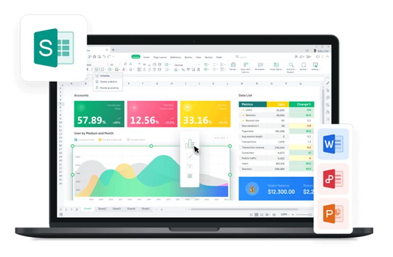
Best Alternative to Microsoft Excel - WPS Office

WPS Office is a free and open-source office suite that is a good alternative to Microsoft Office. It includes a word processor, spreadsheet, presentation software, and a PDF viewer.
Download for free: WPS Office offers a free version with most essential features. The paid version, WPS Office Premium, includes additional features such as cloud storage, templates, and advanced security.
Compatibility: WPS Office maintains full compatibility with Microsoft Office features, formulas, and macros. This means that you can open and edit Microsoft Office files in WPS Office without any problems.
Here are some of the pros and cons of WPS Office:
Pros:
Free and open-source
Full compatibility with Microsoft Office
Includes a variety of features, including a word processor, spreadsheet, presentation software, and a PDF viewer
Easy to use
Cons:
The free version has some limitations, such as the number of documents that you can create and save
The interface is not as user-friendly as Microsoft Office
Overall, WPS Office is a good alternative to Microsoft Office if you are looking for a free and open-source office suite. It is compatible with Microsoft Office files and includes a variety of features.


FAQs about Pivot Charts in Excel
Can I create a Pivot Chart with real-time data updates?
Yes, you can create a Pivot Chart with real-time data updates in Excel. However, Excel itself doesn't provide native real-time data updating for Pivot Charts. The updating of data in a Pivot Chart typically requires a manual refresh or an automatic refresh triggered by certain actions or time intervals.
How can I add trendlines to a Pivot Chart?
Adding Trendlines to a Pivot Chart in Excel
Step 1. Select Data Series: Click the data in your Pivot Chart.
Step 2. Insert Trendline: Right-click, choose "Add Trendline."

Step 3. Choose Trendline Type: Select linear, exponential, etc.

Step 4. Customize: Adjust line style and color.
Step 5. Display Equation: Show equation and R-squared if needed.
Step 6. Done: Close the trendline options.
Now your Pivot Chart displays trendlines for data trend analysis.
Can I use Pivot Charts in Excel Online?
Yes, you can use Pivot Charts in Excel Online. Microsoft has extended the functionality of Excel Online to include Pivot Charts, allowing you to create and work with them directly in your web browser.
Summary
This guide offered clear steps to excel at Pivot Charts in Excel, covering creation, customization, trendlines, and real-time updates. It highlighted WPS Office as a potent alternative. From basic charts to advanced dashboards, the guide ensured easy learning for all skill levels, enhancing data analysis with visual insights.

'%3e%3cpath%20d='M19.9911%204.11386V6.471H18.5894C18.0775%206.471%2017.7322%206.57814%2017.5536%206.79243C17.3751%207.00671%2017.2858%207.32814%2017.2858%207.75671V9.44421H19.9019L19.5536%2012.0871H17.2858V18.8639H14.5536V12.0871H12.2769V9.44421H14.5536V7.49779C14.5536%206.39064%2014.8632%205.53201%2015.4822%204.92189C16.1013%204.31177%2016.9257%204.00671%2017.9554%204.00671C18.8304%204.00671%2019.509%204.04243%2019.9911%204.11386Z'%20fill='%23333333'/%3e%3c/g%3e%3cdefs%3e%3cclipPath%20id='clip0_2938_8199'%3e%3crect%20width='16'%20height='16'%20fill='white'%20transform='translate(8%204.00671)'/%3e%3c/clipPath%3e%3c/defs%3e%3c/svg%3e)
'%3e%3cpath%20d='M17.5237%2010.7813L23.4811%204H22.0699L16.8949%209.88693L12.7648%204H8L14.2469%2012.9029L8%2020.0133H9.4112L14.8725%2013.7952L19.2352%2020.0133H24M9.92053%205.04213H12.0885L22.0688%2019.0224H19.9003'%20fill='%23333333'/%3e%3c/g%3e%3cdefs%3e%3cclipPath%20id='clip0_2938_8200'%3e%3crect%20width='16'%20height='16.0134'%20fill='white'%20transform='translate(8%204)'/%3e%3c/clipPath%3e%3c/defs%3e%3c/svg%3e)


