Free All-in-One Office Suite with PDF Editor

Edit Word, Excel, and PPT for FREE.
Read, edit, and convert PDFs with the powerful PDF toolkit.
Microsoft-like interface, easy to use.
Windows • MacOS • Linux • iOS • Android

Catalog
How to add drop-down options in Excel column (Easy Steps)
If you want to make sure that users choose an item from a list rather than entering their own values, drop-down lists in Excel might be useful. Users can choose an option from a list of possibilities when using the data validation feature of an Excel drop down list. By adding scenarios and making a spreadsheet more dynamic, it may be very helpful when undertaking financial modelling and analysis. The time it could take to enter data into a spreadsheet can be significantly decreased by using a dropdown list in Excel. Thankfully, making a dropdown list in Excel is fairly simple. There are a number ways to achieve this, ranging from easy to complex. In this post, you'll discover all possible approaches.
Create a drop-down list in excel online, 2016 and 2019
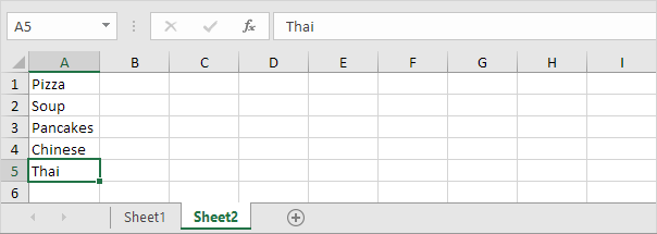
1.Write the things you wish to appear in the drop-down list on the second sheet.
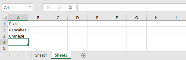
2. Choose cell B1 on the first sheet.

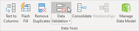
3. Click Data Validation under the Data Tools section of the Data tab.
4. Click List in the Allow box.
5. The range A1:A3 on Sheet2 can be chosen by clicking on the Source box.
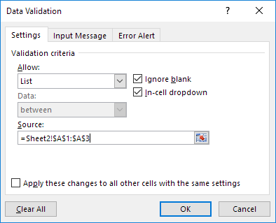
6. Click ok.

Dynamic drop-down list in excel
1.Choose cell B1 on the first sheet..
2. Click Data Validation under the Data Tools section of the Data tab.
3. Click List in the Allow box.
4. Enter the following formula by clicking the Source box: =OFFSET(Sheet2!$A$1,0,0, COUNTA(Sheet2!$A:$A),1)
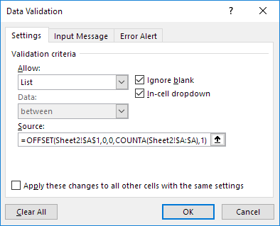
5. Click ok.
6.Simply add a new item to the list's conclusion on the second sheet.

How to remove a drop-down list in excel
1.Choose the cell that contains the drop-down menu.

2. Click Data Validation under the Data Tools section of the Data tab.
3. Click on clear all.
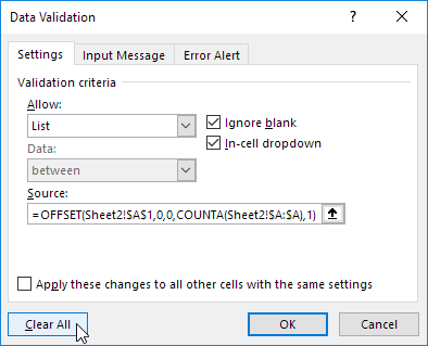
Before clicking Clear All, make sure Apply these changes to all other cells with the same settings is selected in order to erase all other drop-down lists with the same settings.
4. Click ok.
Note: This article was an attemot to make you understand how to add drop-down options in excel, dynamic drop-down list and how to remove drop-down list in excel online, 2016 and 2019. You can also do this on both windows and mac.
To get the newest version of WPS Office, you must first access this operating interface.
You just need to have a little understanding of how and which way things work and you are good to go. With having this basic knowledge or information of how to use it, you can also access and use different other options on excel or spreadsheet. Also, it is very similar to Word or Document. So, in a way, if you learn one thing, like Excel, you can automatically learn how to use Word as well because both of them are very similar in so many ways. If you want to know more about WPS Office, you can download WPS Office to access, Word, Excel, PowerPoint for free.
Also Read:
- 1. Add drop down list excel with multiple selection
- 2. Add a drop down list in Excel with multiple selections
- 3. How to add a calendar template in Excel with drop-down list (2022 Free Templates)
- 4. How to insert drop down list excel
- 5. How to change drop down list in Excel
- 6. How to Add Drop Down in Excel Online


15 years of office industry experience, tech lover and copywriter. Follow me for product reviews, comparisons, and recommendations for new apps and software.
